SEA-AD Multiregion taxonomy and snRNASeq analysis: clustering and annotations

Alzheimer’s disease (AD) is characterized by the progressive accumulation of amyloid-beta (Aβ) plaques and hyperphosphorylated tau (pTau) tangles across brain regions. While these regions differ in architecture, function, and susceptibility to pathology, many share common cellular populations. The SEA-AD Multiregion Taxonomy was developed to provide a unified cellular framework for studying cellular vulnerability and molecular change across the full arc of canonical AD progression.

This taxonomy is derived from a multimodal dataset generated from 84 deeply characterized donors spanning the full spectrum of AD pathology. The dataset presented here contains approximately 6 million high-quality nuclei from single-nucleus RNA-seq and Multiome profiling, along with an additional 2.6 million nuclei that did not pass quality-control criteria. These data were generated alongside approximately 1 million single-nucleus ATAC-seq profiles, which informed multimodal analyses but are not included in the resources described here. Single-nucleus profiling was performed across ten brain regions: medial entorhinal cortex (MEC), lateral entorhinal cortex (LEC), hippocampus (HIP), inferior temporal gyrus (ITG), middle temporal gyrus (MTG), superior temporal gyrus (STG), dorsolateral prefrontal cortex (BA9), frontal insula (FI), angular gyrus (AnG), and primary visual cortex (V1C). Nuclei were mapped to an expanded reference taxonomy comprising 207 cell types, organized into 28 subclasses and 3 major cellular classes, including both broadly shared and regionally specialized populations. Cell type names are harmonized between studies; for example, Sst 25 from Gabitto, Travaglini et al. (2024) and Sst 25 in this taxonomy refer to the same cell population.

To generate this taxonomy, nuclei were subjected to standardized quality control, integrated across regions and modalities, and hierarchically mapped using deep-learning approaches based on scVI and scANVI. The resulting taxonomy provides consistent cell-type nomenclature across SEA-AD resources while preserving region-specific cellular specializations found in allocortical and neocortical regions. Spatial transcriptomic datasets were additionally used to anatomically localize newly defined excitatory populations within the hippocampus and entorhinal cortex.

The notebook presented here demonstrates how to access and visualize taxonomy annotations, cell type metadata, donor information, brain region annotations, and AD-associated cellular changes from the SEA-AD multiregional dataset. These examples focus on precomputed metadata accessible through the Allen Brain Cell Atlas Access package. Additional data, including links to raw sequencing, spatial transcriptomic, and neuropathology data, are available at SEA-AD.org.

%matplotlib inline

import pandas as pd
from pathlib import Path
import numpy as np
import matplotlib.pyplot as plt
from typing import Tuple, Optional

from abc_atlas_access.abc_atlas_cache.abc_project_cache import AbcProjectCache

We will interact with the data using the AbcProjectCache. This cache object downloads data requested by the user, tracks which files have already been downloaded to your local system, and serves the path to the requested data on disk. For metadata, the cache can also directly serve up a Pandas DataFrame. See the getting_started notebook for more details on using the cache including installing it if it has not already been.

Change the download_base variable to where you would like to download the data in your system or a location where a cache is already available.

download_base = Path('../../data/allen-brain-cell-atlas-staging/')
abc_cache = AbcProjectCache.from_cache_dir(
   download_base
)

abc_cache.current_manifest

'releases/20260711/manifest.json'

Data overview

Below we list the metadata and gene expression files for each of the directories that make up this dataset:

• SEA-AD-Multiregion-10X

• SEA-AD-Multiregion-taxonomy

print("SEA-AD-10X: gene expression data (h5ad)\n\t", abc_cache.list_expression_matrix_files(directory='SEA-AD-Multiregion-10X'))
print("SEA-AD-Multiregion-10X: metadata (csv)\n\t", abc_cache.list_metadata_files(directory='SEA-AD-Multiregion-10X'))

SEA-AD-10X: gene expression data (h5ad)
	 ['AnG-10X/log2', 'AnG-10X/raw', 'DFC-10X/log2', 'DFC-10X/raw', 'FI-10X/log2', 'FI-10X/raw', 'HIP-10X/log2', 'HIP-10X/raw', 'ITG-10X/log2', 'ITG-10X/raw', 'LEC-10X/log2', 'LEC-10X/raw', 'MEC-10X/log2', 'MEC-10X/raw', 'MTG-10X/log2', 'MTG-10X/raw', 'STG-10X/log2', 'STG-10X/raw', 'V1C-10X/log2', 'V1C-10X/raw']
SEA-AD-Multiregion-10X: metadata (csv)
	 ['cell_metadata', 'disease', 'donor', 'example_gene_expression', 'gene', 'library', 'value_sets']

We will also use metadata from the SEA-AD-Multiregion-taxonomy directory. Below is the list of available files:

print("SEA-AD-Multiregion-taxonomy: metadata (csv)\n\t", abc_cache.list_metadata_files(directory='SEA-AD-Multiregion-taxonomy'))

SEA-AD-Multiregion-taxonomy: metadata (csv)
	 ['cell_2d_embedding_coordinates', 'cell_to_cluster_membership', 'cluster', 'cluster_annotation_term', 'cluster_annotation_term_set', 'cluster_to_cluster_annotation_membership']

Cell metadata

Essential cell metadata is stored as a CSV file that we load as a Pandas DataFrame. Each row represents one cell indexed by a cell label. The cell label is the concatenation of barcode and name of the sample. In this context, the sample is the barcoded cell sample that represents a single load into one port of the 10x Chromium. Note that cell barcodes are only unique within a single barcoded cell sample and that the same barcode can be reused exp_component_name is an alternative cell identifier that indexes some of the data hosted at SEA-AD.org.

Each cell is associated with a library label, donor label, alignment_job_id, feature_matrix_label and dataset_label identifying which data package this cell is part of. This metadata file will be combined with other metadata files that come with this package to add information associated with the donor, UMAP coordinates, taxonomy assignments, and more.

Below, we load the first of the metadata used in this tutorial. This represents the cell metadata for the aligned dataset.

The command we use below both downloads the data if it is not already available in the local cache and loads the data as a Pandas DataFrame. This pattern of loading metadata is repeated throughout the tutorials.

cell = abc_cache.get_metadata_dataframe(
    directory='SEA-AD-Multiregion-10X',
    file_name='cell_metadata'
).set_index('cell_label')
print("Number of cells = ", len(cell))
cell.head()

cell_metadata.csv: 100%|██████████| 1.64G/1.64G [02:44<00:00, 9.98MMB/s]   
/Users/chris.morrison/src/abc_atlas_access/src/abc_atlas_access/abc_atlas_cache/abc_project_cache.py:643: DtypeWarning: Columns (4) have mixed types. Specify dtype option on import or set low_memory=False.
  return pd.read_csv(path, **kwargs)

Number of cells =  8641342

	cell_barcode	barcoded_cell_sample_label	library_label	alignment_job_id	doublet_score	umi_count	donor_label	exp_component_name	feature_matrix_label	dataset_label
cell_label
AAACAGCCACTGGCTG-2001_A08	AAACAGCCACTGGCTG	2001_A08	L8XR_231221_02_D02	1322484698	0.184615	54020.0	H21.33.001	AAACAGCCACTGGCTG-L8XR_231221_02_D02-1322484698	AnG-10X	SEA-AD-Multiregion-10X
AAACAGCCAGGTTATT-2001_A08	AAACAGCCAGGTTATT	2001_A08	L8XR_231221_02_D02	1322484698	0.060606	4438.0	H21.33.001	AAACAGCCAGGTTATT-L8XR_231221_02_D02-1322484698	AnG-10X	SEA-AD-Multiregion-10X
AAACAGCCATTCCTCG-2001_A08	AAACAGCCATTCCTCG	2001_A08	L8XR_231221_02_D02	1322484698	0.276923	66285.0	H21.33.001	AAACAGCCATTCCTCG-L8XR_231221_02_D02-1322484698	AnG-10X	SEA-AD-Multiregion-10X
AAACATGCAATGCCTA-2001_A08	AAACATGCAATGCCTA	2001_A08	L8XR_231221_02_D02	1322484698	0.060606	6019.0	H21.33.001	AAACATGCAATGCCTA-L8XR_231221_02_D02-1322484698	AnG-10X	SEA-AD-Multiregion-10X
AAACATGCACCTCACC-2001_A08	AAACATGCACCTCACC	2001_A08	L8XR_231221_02_D02	1322484698	0.181818	48653.0	H21.33.001	AAACATGCACCTCACC-L8XR_231221_02_D02-1322484698	AnG-10X	SEA-AD-Multiregion-10X

We can use pandas groupby function to see how many unique items are associated for each field and list them out if the number of unique items is small.

def print_column_info(df):
    
    for c in df.columns:
        grouped = df[[c]].groupby(c).count()
        members = ''
        if len(grouped) < 30:
            members = str(list(grouped.index))
        print("Number of unique %s = %d %s" % (c, len(grouped), members))

print_column_info(cell)

Number of unique cell_barcode = 3767416 
Number of unique barcoded_cell_sample_label = 908 
Number of unique library_label = 908 
Number of unique alignment_job_id = 913 
Number of unique doublet_score = 2792 
Number of unique umi_count = 177044 
Number of unique donor_label = 84 
Number of unique exp_component_name = 8641342 
Number of unique feature_matrix_label = 10 ['AnG-10X', 'DFC-10X', 'FI-10X', 'HIP-10X', 'ITG-10X', 'LEC-10X', 'MEC-10X', 'MTG-10X', 'STG-10X', 'V1C-10X']
Number of unique dataset_label = 1 ['SEA-AD-Multiregion-10X']

Donor, Library, and Disease metadata

The first two associated metadata we load are the donor, library, and disease tables. The donor table includes donor demographics such as species, age, sex, race, and education, along with brain tissue metrics such as pH, postmortem interval (PMI), and fresh brain weight. This table also indicates which study a donor was enrolled in (ACT or ADRC). The library table contains information on 10X methods and brain region of interest the tissue was extracted from. The disease table contains disease progression metrics and other pathology data. Definitions of many of these columns can be found here.

donor = abc_cache.get_metadata_dataframe(
    directory='SEA-AD-Multiregion-10X',
    file_name='donor',
).set_index('donor_label')

donor

donor.csv: 100%|██████████| 17.1k/17.1k [00:00<00:00, 235kMB/s]

	donor_species	species_scientific_name	species_genus	donor_sex	donor_gender	donor_age	donor_age_value	donor_age_unit	Race (choice=White)	Race (choice=Black/ African American)	...	Race (choice=Other)	Hispanic/Latino	specify other race	Highest level of education	Years of education	PMI	Fresh Brain Weight	Brain pH	Primary Study Name	donor_race
donor_label
H19.33.004	NCBITaxon:9606	Homo sapiens	Human	Female	Female	80 yrs	80	years	Checked	Unchecked	...	Unchecked	No	NaN	Bachelors	17	8.133333	1035.0	7.0	ACT	White
H20.33.001	NCBITaxon:9606	Homo sapiens	Human	Male	Male	82 yrs	82	years	Checked	Unchecked	...	Unchecked	No	NaN	Bachelors	16	7.700000	1338.0	6.8	ACT	White
H20.33.002	NCBITaxon:9606	Homo sapiens	Human	Female	Female	97 yrs	97	years	Checked	Unchecked	...	Unchecked	No	NaN	High School	12	4.333333	1078.0	7.3	ACT	White
H20.33.004	NCBITaxon:9606	Homo sapiens	Human	Male	Male	86 yrs	86	years	Checked	Unchecked	...	Unchecked	No	NaN	Trade School/ Tech School	15	8.833333	1261.0	6.7	ACT	White
H20.33.005	NCBITaxon:9606	Homo sapiens	Human	Female	Female	99 yrs	99	years	Checked	Unchecked	...	Unchecked	No	NaN	High School	12	7.600000	1003.0	6.8	ACT	White
...	...	...	...	...	...	...	...	...	...	...	...	...	...	...	...	...	...	...	...	...	...
H21.33.043	NCBITaxon:9606	Homo sapiens	Human	Female	Female	95 yrs	95	years	Checked	Unchecked	...	Unchecked	No	NaN	Bachelors	16	4.400000	1082.0	6.6	ACT	White
H21.33.044	NCBITaxon:9606	Homo sapiens	Human	Female	Female	88 yrs	88	years	Checked	Unchecked	...	Unchecked	No	NaN	Trade School/ Tech School	15	7.000000	1168.0	6.6	ACT	White
H21.33.045	NCBITaxon:9606	Homo sapiens	Human	Female	Female	94 yrs	94	years	Unchecked	Unchecked	...	Unchecked	No	NaN	High School	12	4.000000	925.0	7.2	ADRC Clinical Core	Asian
H21.33.046	NCBITaxon:9606	Homo sapiens	Human	Male	Male	97 yrs	97	years	Checked	Unchecked	...	Unchecked	No	NaN	Professional	17	7.000000	1159.0	6.4	ACT	White
H21.33.047	NCBITaxon:9606	Homo sapiens	Human	Female	Male	90 yrs	90	years	Checked	Unchecked	...	Unchecked	No	NaN	Professional	21	4.400000	1168.0	7.2	ACT	White

84 rows × 24 columns

Next we load the library metadata. The information we will primarily use from this table are the region of interest that each library is associated with

library = abc_cache.get_metadata_dataframe(
    directory='SEA-AD-Multiregion-10X',
    file_name='library'
).set_index('library_label')
library

library.csv: 100%|██████████| 117k/117k [00:00<00:00, 564kMB/s]  

	library_method	barcoded_cell_sample_label	enrichment_population	cell_specimen_type	region_of_interest_label	region_of_interest_name	parcellation_term_identifier	Brain Region	donor_label
library_label
L8XR_231221_02_D02	10xMultiome;GEX	2001_A08	70% NeuN+, 30% NeuN-	Nuclei	AnG	angular gyrus	DHBA:12136	AnG	H21.33.001
L8XR_231130_21_B02	10xMultiome;GEX	1963_A06	70% NeuN+, 30% NeuN-	Nuclei	AnG	angular gyrus	DHBA:12136	AnG	H21.33.002
L8XR_231116_02_B08	10xMultiome;GEX	1957_A08	70% NeuN+, 30% NeuN-	Nuclei	AnG	angular gyrus	DHBA:12136	AnG	H20.33.035
L8XR_231130_21_E02	10xMultiome;GEX	1967_B09	70% NeuN+, 30% NeuN-	Nuclei	AnG	angular gyrus	DHBA:12136	AnG	H21.33.028
L8XR_231221_02_G02	10xMultiome;GEX	2001_C08	70% NeuN+, 30% NeuN-	Nuclei	AnG	angular gyrus	DHBA:12136	AnG	H21.33.004
...	...	...	...	...	...	...	...	...	...
L8XR_240530_01_G08	10xMultiome;GEX	2252_A07	70% NeuN+, 30% NeuN-	Nuclei	FI	frontal agranular insular cortex (area FI)	DHBA:10329	FI	H20.33.018
L8XR_240607_02_A04	10xMultiome;GEX	2252_B07	70% NeuN+, 30% NeuN-	Nuclei	FI	frontal agranular insular cortex (area FI)	DHBA:10329	FI	H20.33.028
L8XR_240607_02_F04	10xMultiome;GEX	2252_C07	70% NeuN+, 30% NeuN-	Nuclei	FI	frontal agranular insular cortex (area FI)	DHBA:10329	FI	H20.33.033
L8XR_240620_01_F09	10xMultiome;GEX	2284_C09	70% NeuN+, 30% NeuN-	Nuclei	FI	frontal agranular insular cortex (area FI)	DHBA:10329	FI	H20.33.037
L8XR_240801_02_F09	10xMultiome;GEX	2351_B09	70% NeuN+, 30% NeuN-	Nuclei	FI	frontal agranular insular cortex (area FI)	DHBA:10329	FI	H21.33.026

908 rows × 9 columns

Finally we load the disease data containing disease progression information.

disease = abc_cache.get_metadata_dataframe(
    directory='SEA-AD-Multiregion-10X',
    file_name='disease'
).set_index('donor_label')
disease

disease.csv: 100%|██████████| 14.4k/14.4k [00:00<00:00, 94.3kMB/s]

	Overall AD neuropathological Change	Thal	Braak	CERAD score	Overall CAA Score	Highest Lewy Body Disease	Total Microinfarcts (not observed grossly)	Total microinfarcts in screening sections	Atherosclerosis	Arteriolosclerosis	...	Cognitive Status	Last CASI Score	Interval from last CASI in months	Last MMSE Score	Interval from last MMSE in months	Last MOCA Score	Interval from last MOCA in months	APOE Genotype	Severely Affected Donor	CPS_Global
donor_label
H19.33.004	Not AD	Thal 0	Braak IV	Absent	Not identified	Not Identified (olfactory bulb not assessed)	1	1	Mild	Moderate	...	No dementia	85.0	3.5	25.0	3.5	NaN	NaN	3/3	N	0.102055
H20.33.001	Low	Thal 2	Braak IV	Sparse	Not identified	Not Identified (olfactory bulb not assessed)	0	0	Mild	Mild	...	No dementia	97.0	18.2	28.0	18.2	NaN	NaN	3/3	N	0.390107
H20.33.002	Not AD	Thal 0	Braak IV	Absent	Not identified	Limbic (Transitional)	0	0	Moderate	Moderate	...	No dementia	93.0	46.1	33.0	22.6	NaN	NaN	2/3	N	0.081825
H20.33.004	High	Thal 5	Braak V	Frequent	Moderate	Neocortical (Diffuse)	0	0	Mild	Severe	...	Dementia	80.0	55.7	25.0	55.7	NaN	NaN	3/4	N	0.754141
H20.33.005	Intermediate	Thal 3	Braak IV	Moderate	Moderate	Not Identified (olfactory bulb not assessed)	2	2	Mild	Moderate	...	No dementia	94.0	24.2	29.0	24.2	NaN	NaN	2/3	N	0.276006
...	...	...	...	...	...	...	...	...	...	...	...	...	...	...	...	...	...	...	...	...	...
H21.33.043	Low	Thal 4	Braak II	Sparse	Not identified	Not Identified (olfactory bulb assessed)	1	0	Moderate	Moderate	...	Dementia	97.0	35.1	29.0	35.1	NaN	NaN	3/3	N	0.580067
H21.33.044	Intermediate	Thal 3	Braak VI	Frequent	Moderate	Not Identified (olfactory bulb not assessed)	9	9	Mild	Severe	...	Dementia	81.0	8.9	21.0	8.9	NaN	NaN	3/3	N	0.731159
H21.33.045	High	Thal 4	Braak VI	Frequent	Moderate	Limbic (Transitional)	0	0	Moderate	Moderate	...	Dementia	NaN	NaN	17.0	65.3	NaN	NaN	3/4	Y	0.962116
H21.33.046	High	Thal 4	Braak V	Moderate	Moderate	Neocortical (Diffuse)	0	0	Mild	Severe	...	Dementia	81.0	22.3	22.0	22.3	NaN	NaN	3/3	N	0.752803
H21.33.047	Intermediate	Thal 2	Braak V	Frequent	Not identified	Neocortical (Diffuse)	1	1	Moderate	Moderate	...	No dementia	90.0	7.4	26.0	7.4	NaN	NaN	3/3	N	0.259830

84 rows × 21 columns

We combine the donor, library, and disease tables into an extended cell metadata table.

cell_extended = cell.join(donor, on='donor_label')
cell_extended = cell_extended.join(library, on='library_label', rsuffix='_library_table')
cell_extended = cell_extended.join(disease, on='donor_label', rsuffix='_disease')

del cell

We use the groupby function to show the number of cells for one of disease data columns. Change this to any other column to get counts by any of the various metadata.

cell_extended.groupby('region_of_interest_name')[['region_of_interest_label']].count()

	region_of_interest_label
region_of_interest_name
angular gyrus	389804
dorsolateral prefrontal cortex	1807513
frontal agranular insular cortex (area FI)	321843
hippocampus (hippocampal formation)	307789
inferior temporal gyrus	626792
lateral (anterior) entorhinal cortex	239721
medial (posterior) entorhinal cortex	1485051
middle temporal gyrus	1861334
primary visual cortex (striate cortex, area V1/17)	867151
superior temporal gyrus	734344

We can use the group by functionality to group the cells by cognitive status.

cell_extended.groupby('Cognitive Status')[['library_label']].count().rename(columns={'library_label': 'number_of_cells'})

	number_of_cells
Cognitive Status
Dementia	3943893
No dementia	4697449

Adding color and feature order

Each major feature in the donor and library table is associated with unique colors and an ordering with the set of values. Below we load the value_sets DataFrame which is a mapping from the various value in the donor and species tables to those colors and orderings. We incorporate these values into the cell metadata table.

value_sets = abc_cache.get_metadata_dataframe(
    directory='SEA-AD-Multiregion-10X',
    file_name='value_sets'
).set_index('label')
value_sets

value_sets.csv: 100%|██████████| 15.6k/15.6k [00:00<00:00, 111kMB/s] 

	field	table	color_hex_triplet	order	description	external_identifier
label
2/2	APOE Genotype	disease	#fdd4c2	1	NaN	NaN
2/3	APOE Genotype	disease	#fca082	2	NaN	NaN
2/4	APOE Genotype	disease	#fb6a4a	3	NaN	NaN
3/3	APOE Genotype	disease	#e32f27	4	NaN	NaN
3/4	APOE Genotype	disease	#b21218	5	NaN	NaN
...	...	...	...	...	...	...
FI	region_of_interest_label	library	#008080	7	agranular frontal insular cortex (area FI)	DHBA:10329
STG	region_of_interest_label	library	#006400	8	superior temporal gyrus	DHBA:12140
DFC	region_of_interest_label	library	#00008b	9	dorsolateral prefrontal cortex	DHBA:10173
AnG	region_of_interest_label	library	#00bfff	10	angular gyrus	DHBA:12136
V1C	region_of_interest_label	library	#9932cc	11	primary visual cortex (first visual cortex, st...	DHBA:10269

204 rows × 6 columns

We define a convenience function to add colors for the various values in the data (e.g. unique region of interest or donor sex values).

def extract_value_set(
        cell_metadata_df: pd.DataFrame,
        input_value_set: pd.DataFrame,
        input_value_set_label: str,
        dataframe_column: Optional[str] = None
    ):
    """Add color and order columns to the cell metadata dataframe based on the input
    value set.

    Columns are added as {input_value_set_label}_color and {input_value_set_label}_order.

    Parameters
    ----------
    cell_metadata_df : pd.DataFrame
        DataFrame containing cell metadata.
    input_value_set : pd.DataFrame
        DataFrame containing the value set information.
    input_value_set_label : str
        The the column name to extract color and order information for. will be added to the cell metadata.
    """
    if dataframe_column is None:
        dataframe_column = input_value_set_label
    cell_metadata_df[f'{dataframe_column}_color'] = input_value_set[
        input_value_set['field'] == input_value_set_label
    ].loc[cell_metadata_df[dataframe_column]]['color_hex_triplet'].values
    cell_metadata_df[f'{dataframe_column}_order'] = input_value_set[
        input_value_set['field'] == input_value_set_label
    ].loc[cell_metadata_df[dataframe_column]]['order'].values

Use our function to add the relevant color and order columns to our cell_metadata table.

# Add region of interest color and order
extract_value_set(cell_extended, value_sets, 'region_of_interest_label')
# Add disease color and order
extract_value_set(cell_extended, value_sets, 'APOE Genotype')
extract_value_set(cell_extended, value_sets, 'Arteriolosclerosis')
extract_value_set(cell_extended, value_sets, 'Atherosclerosis')
extract_value_set(cell_extended, value_sets, 'Braak')
extract_value_set(cell_extended, value_sets, 'CERAD score')
extract_value_set(cell_extended, value_sets, 'Cognitive Status')
extract_value_set(cell_extended, value_sets, 'LATE')
extract_value_set(cell_extended, value_sets, 'Highest Lewy Body Disease')
extract_value_set(cell_extended, value_sets, 'Overall AD neuropathological Change')
extract_value_set(cell_extended, value_sets, 'Severely Affected Donor')
extract_value_set(cell_extended, value_sets, 'Thal')
# Add donor sex/gender color and order
extract_value_set(cell_extended, value_sets, 'donor_sex')
extract_value_set(cell_extended, value_sets, 'donor_gender')
# Add race
extract_value_set(cell_extended, value_sets, 'donor_race')
cell_extended.head()

	cell_barcode	barcoded_cell_sample_label	library_label	alignment_job_id	doublet_score	umi_count	donor_label	exp_component_name	feature_matrix_label	dataset_label	...	Severely Affected Donor_color	Severely Affected Donor_order	Thal_color	Thal_order	donor_sex_color	donor_sex_order	donor_gender_color	donor_gender_order	donor_race_color	donor_race_order
cell_label
AAACAGCCACTGGCTG-2001_A08	AAACAGCCACTGGCTG	2001_A08	L8XR_231221_02_D02	1322484698	0.184615	54020.0	H21.33.001	AAACAGCCACTGGCTG-L8XR_231221_02_D02-1322484698	AnG-10X	SEA-AD-Multiregion-10X	...	#fb6a4a	1	#fc8161	3	#ADC4C3	2	#ADC4C3	2	#f7f184	125
AAACAGCCAGGTTATT-2001_A08	AAACAGCCAGGTTATT	2001_A08	L8XR_231221_02_D02	1322484698	0.060606	4438.0	H21.33.001	AAACAGCCAGGTTATT-L8XR_231221_02_D02-1322484698	AnG-10X	SEA-AD-Multiregion-10X	...	#fb6a4a	1	#fc8161	3	#ADC4C3	2	#ADC4C3	2	#f7f184	125
AAACAGCCATTCCTCG-2001_A08	AAACAGCCATTCCTCG	2001_A08	L8XR_231221_02_D02	1322484698	0.276923	66285.0	H21.33.001	AAACAGCCATTCCTCG-L8XR_231221_02_D02-1322484698	AnG-10X	SEA-AD-Multiregion-10X	...	#fb6a4a	1	#fc8161	3	#ADC4C3	2	#ADC4C3	2	#f7f184	125
AAACATGCAATGCCTA-2001_A08	AAACATGCAATGCCTA	2001_A08	L8XR_231221_02_D02	1322484698	0.060606	6019.0	H21.33.001	AAACATGCAATGCCTA-L8XR_231221_02_D02-1322484698	AnG-10X	SEA-AD-Multiregion-10X	...	#fb6a4a	1	#fc8161	3	#ADC4C3	2	#ADC4C3	2	#f7f184	125
AAACATGCACCTCACC-2001_A08	AAACATGCACCTCACC	2001_A08	L8XR_231221_02_D02	1322484698	0.181818	48653.0	H21.33.001	AAACATGCACCTCACC-L8XR_231221_02_D02-1322484698	AnG-10X	SEA-AD-Multiregion-10X	...	#fb6a4a	1	#fc8161	3	#ADC4C3	2	#ADC4C3	2	#f7f184	125

5 rows × 94 columns

UMAP spatial embedding

Now that we’ve merged our donor and library metadata into the main cells data, our next step is to plot these values in the Uniform Manifold Approximation and Projection (UMAP) for cells in the dataset. The UMAP is a dimension reduction technique that can be used for visualizing and exploring large-dimension datasets.

Below we load this 2-D embedding for a sub selection of our cells and merge the x-y coordinates into the extended cell metadata we are creating.

cell_2d_embedding_coordinates = abc_cache.get_metadata_dataframe(
    directory='SEA-AD-Multiregion-taxonomy',
    file_name='cell_2d_embedding_coordinates'
).set_index('cell_label')
cell_2d_embedding_coordinates.head()

cell_2d_embedding_coordinates.csv: 100%|██████████| 273M/273M [00:26<00:00, 10.5MMB/s]    

	x	y
cell_label
AAACAGCCACTGGCTG-2001_A08	7.009472	14.111731
AAACAGCCAGGTTATT-2001_A08	-1.319671	-1.221017
AAACAGCCATTCCTCG-2001_A08	17.003418	10.816355
AAACATGCAATGCCTA-2001_A08	17.077744	2.317490
AAACATGCACCTCACC-2001_A08	19.195032	1.132652

After joining the UMAPS coordinates into our full cell metadata table, we’ll subset every 10th cell the full dataset for ease of plotting.

cell_extended = cell_extended.join(cell_2d_embedding_coordinates, how='inner')
cell_extended = cell_extended.sample(frac=1) # shuffle the rows for plotting purposes
plot_cell_extended = cell_extended[::10]

del cell_2d_embedding_coordinates

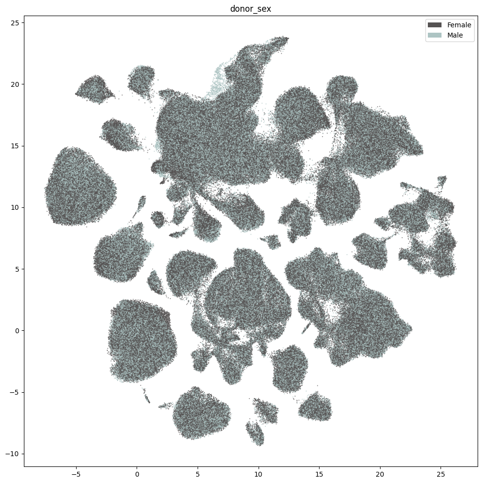
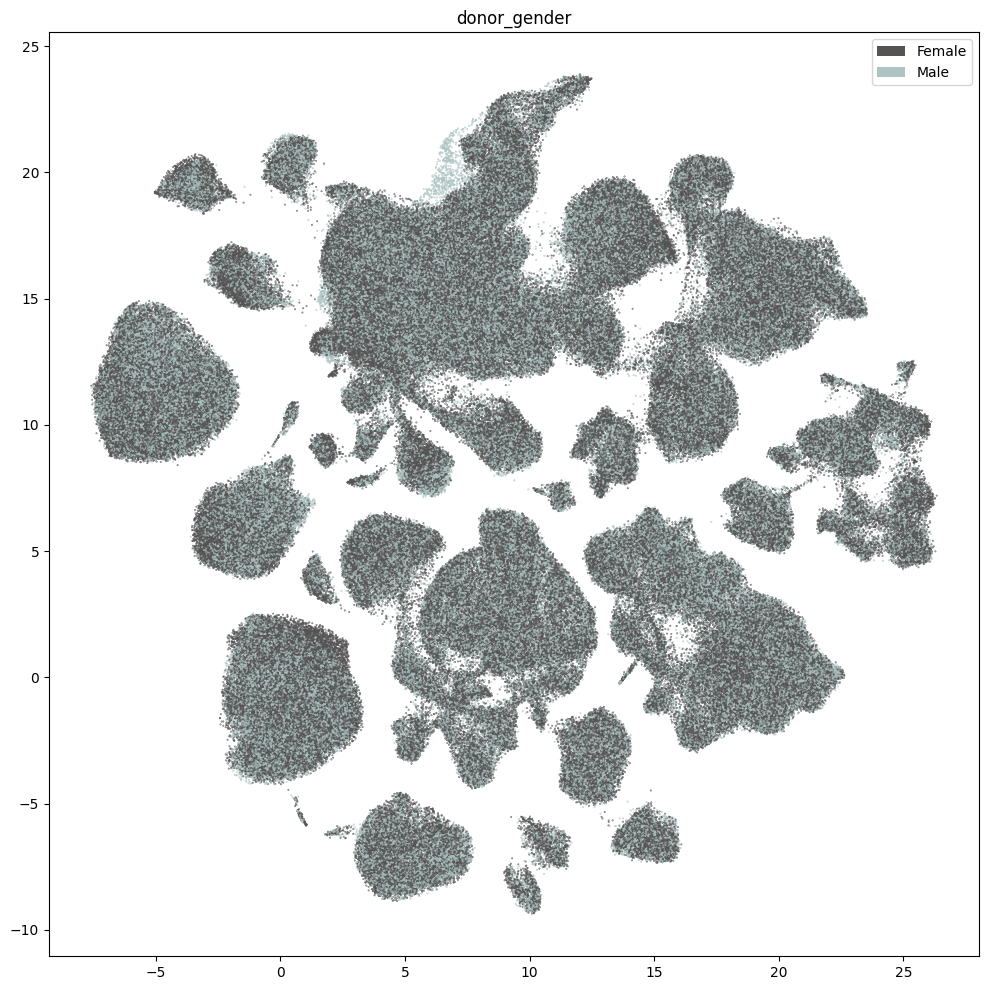
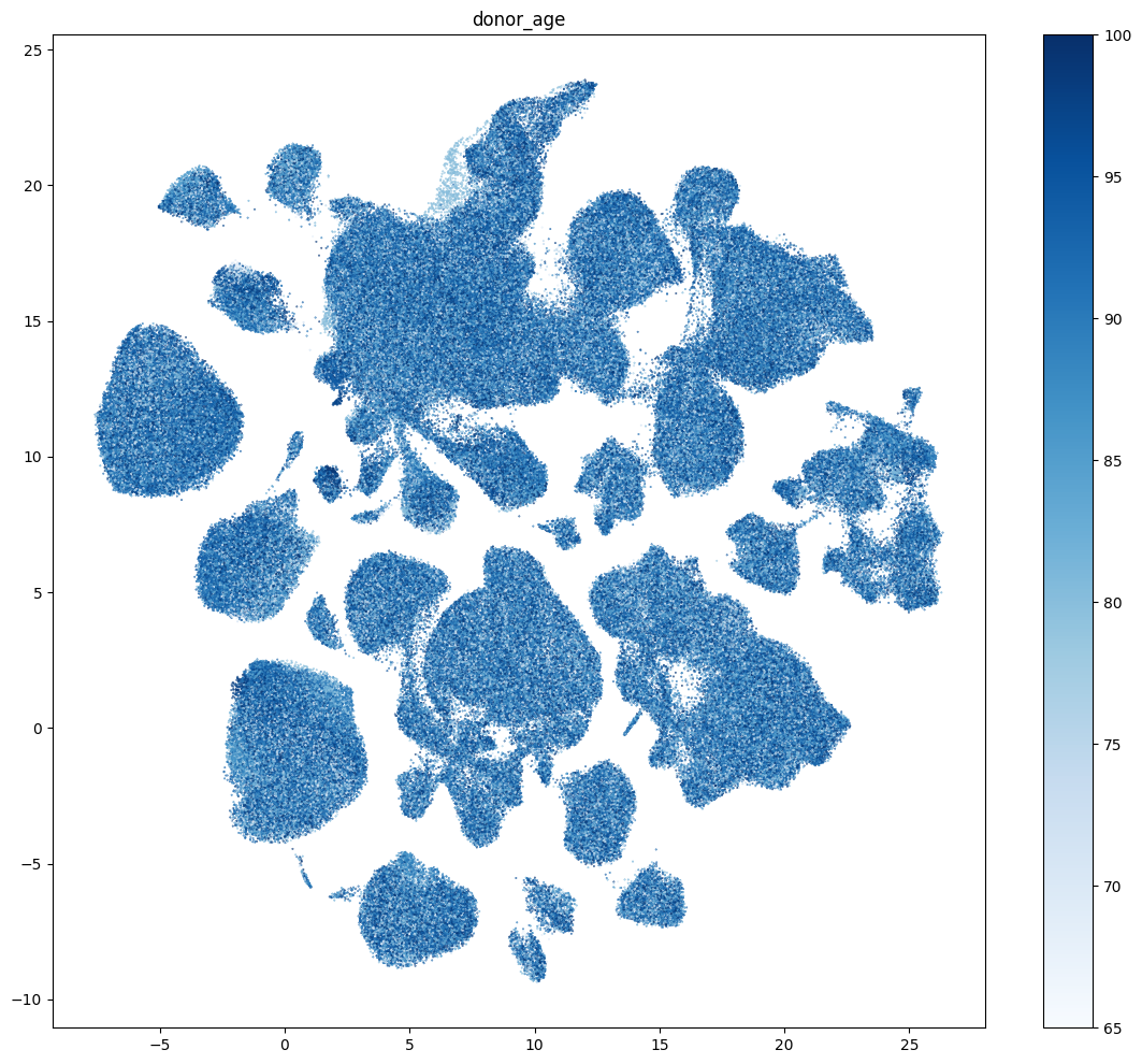
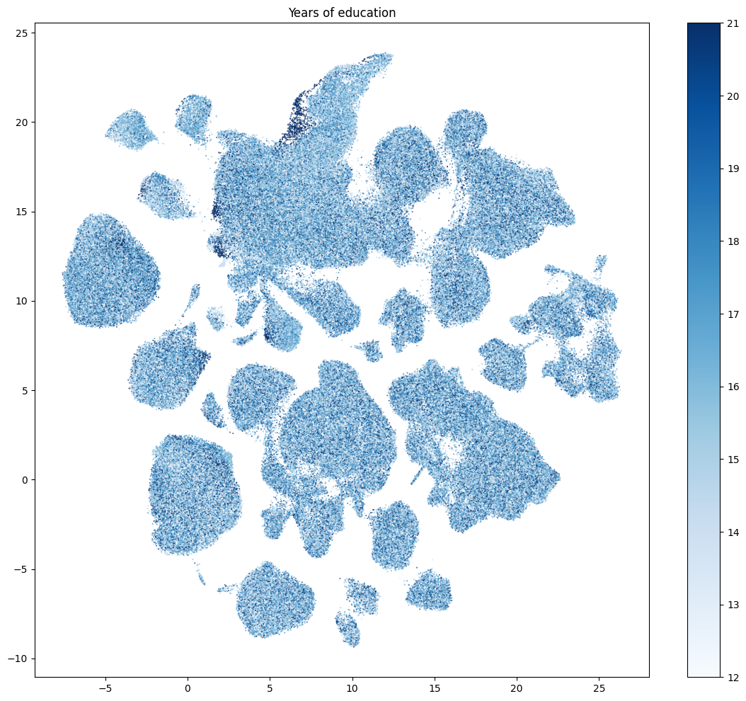
We define a small helper function plot_umap to visualize the cells on the UMAP. In the examples below we will plot associated cell information colorized by donor age, sex, region of interest,etc.

def plot_umap(
    xx: np.ndarray,
    yy: np.ndarray,
    cc: np.ndarray = None,
    val: np.ndarray = None,
    fig_width: float = 8,
    fig_height: float = 8,
    cmap: Optional[plt.Colormap] = None,
    labels: np.ndarray = None,
    term_orders: np.ndarray = None,
    colorbar: bool = False,
    sizes: np.ndarray = None,
    limit_plot: bool = True,
    fig: plt.Figure = None,
    ax: plt.Axes = None,
 ) -> Tuple[plt.Figure, plt.Axes]:
    """
    Plot a scatter plot of the UMAP coordinates.

    Parameters
    ----------
    xx : array-like
        x-coordinates of the points to plot.
    yy : array-like
        y-coordinates of the points to plot.
    cc : array-like, optional
        colors of the points to plot. If None, the points will be colored by the values in `val`.
    val : array-like, optional
        values of the points to plot. If None, the points will be colored by the values in `cc`.
    fig_width : float, optional
        width of the figure in inches. Default is 8.
    fig_height : float, optional
        height of the figure in inches. Default is 8.
    cmap : str, optional
        colormap to use for coloring the points. If None, the points will be colored by the values in `cc`.
    labels : array-like, optional
        labels for the points to plot. If None, no labels will be added to the plot.
    term_orders : array-like, optional
        order of the labels for the legend. If None, the labels will be ordered by their appearance in `labels`.
    colorbar : bool, optional
        whether to add a colorbar to the plot. Default is False.
    sizes : array-like, optional
        sizes of the points to plot. If None, all points will have the same size.
    """
    if sizes is None:
        sizes = 1
    if fig is None or ax is None:
        fig, ax = plt.subplots()
        fig.set_size_inches(fig_width, fig_height)

    if cmap is not None:
        scatt = ax.scatter(xx, yy, c=val, s=0.5, marker='.', cmap=cmap, alpha=sizes)
    elif cc is not None:
        scatt = ax.scatter(xx, yy, c=cc, s=0.5, marker='.', alpha=sizes)

    if labels is not None:
        from matplotlib.patches import Rectangle
        unique_label_colors = (labels + ',' + cc).unique()
        unique_labels = np.array([label_color.split(',')[0] for label_color in unique_label_colors])
        unique_colors = np.array([label_color.split(',')[1] for label_color in unique_label_colors])

        if term_orders is not None:
            unique_order = term_orders.unique()
            term_order = np.argsort(unique_order)
            unique_labels = unique_labels[term_order]
            unique_colors = unique_colors[term_order]
            
        rects = []
        for color in unique_colors:
            rects.append(Rectangle((0, 0), 1, 1, fc=color))

        legend = ax.legend(rects, unique_labels, loc=1)
        # ax.add_artist(legend)

    if colorbar:
        fig.colorbar(scatt, ax=ax)
    
    return fig, ax

Plot the various donor and library metadata available.

fig, ax = plot_umap(
    plot_cell_extended['x'],
    plot_cell_extended['y'],
    cc=plot_cell_extended['donor_sex_color'],
    labels=plot_cell_extended['donor_sex'],
    term_orders=plot_cell_extended['donor_sex_order'],
    fig_width=12,
    fig_height=12
)
res = ax.set_title("donor_sex")
plt.show()

fig, ax = plot_umap(
    plot_cell_extended['x'],
    plot_cell_extended['y'],
    cc=plot_cell_extended['donor_gender_color'],
    labels=plot_cell_extended['donor_gender'],
    term_orders=plot_cell_extended['donor_gender_order'],
    fig_width=12,
    fig_height=12
)
res = ax.set_title("donor_gender")
plt.show()

fig, ax = plot_umap(
    plot_cell_extended['x'],
    plot_cell_extended['y'],
    val=plot_cell_extended['donor_age_value'],
    cmap=plt.cm.Blues,
    fig_width=14,
    fig_height=12,
    colorbar=True,
)
res = ax.set_title("donor_age")
plt.show()

fig, ax = plot_umap(
    plot_cell_extended['x'],
    plot_cell_extended['y'],
    val=plot_cell_extended['Years of education'],
    cmap=plt.cm.Blues,
    fig_width=14,
    fig_height=12,
    colorbar=True,
)
res = ax.set_title("Years of education")
plt.show()

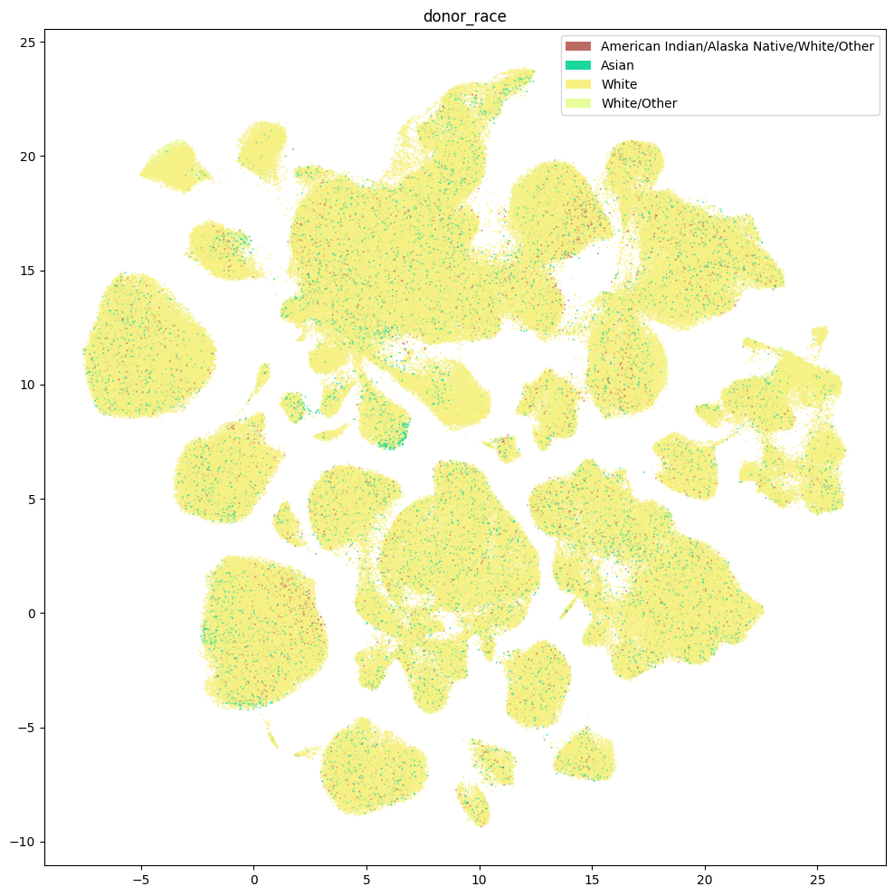
fig, ax = plot_umap(
    plot_cell_extended['x'],
    plot_cell_extended['y'],
    cc=plot_cell_extended['donor_race_color'],
    labels=plot_cell_extended['donor_race'],
    term_orders=plot_cell_extended['donor_race_order'],
    fig_width=12,
    fig_height=12
)
res = ax.set_title("donor_race")
plt.show()

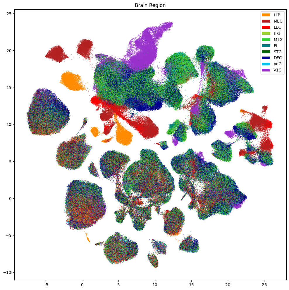
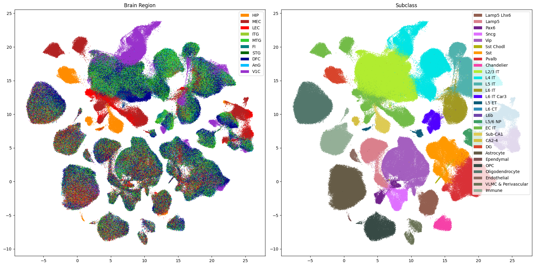
Below we show the region of interest for the cells in the dataset.

fig, ax = plot_umap(
    plot_cell_extended['x'],
    plot_cell_extended['y'],
    cc=plot_cell_extended['region_of_interest_label_color'],
    labels=plot_cell_extended['region_of_interest_label'],
    term_orders=plot_cell_extended['region_of_interest_label_order'],
    fig_width=12,
    fig_height=12
)
res = ax.set_title("Brain Region")
plt.show()

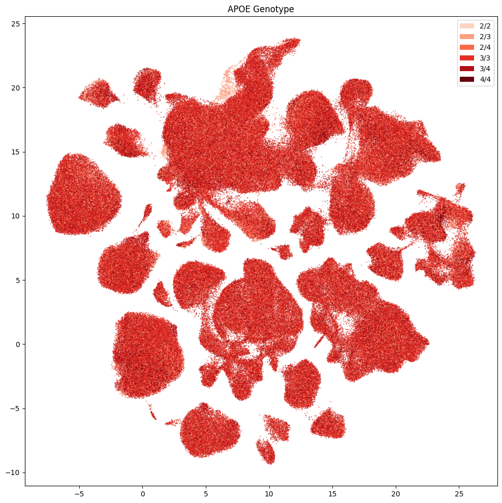
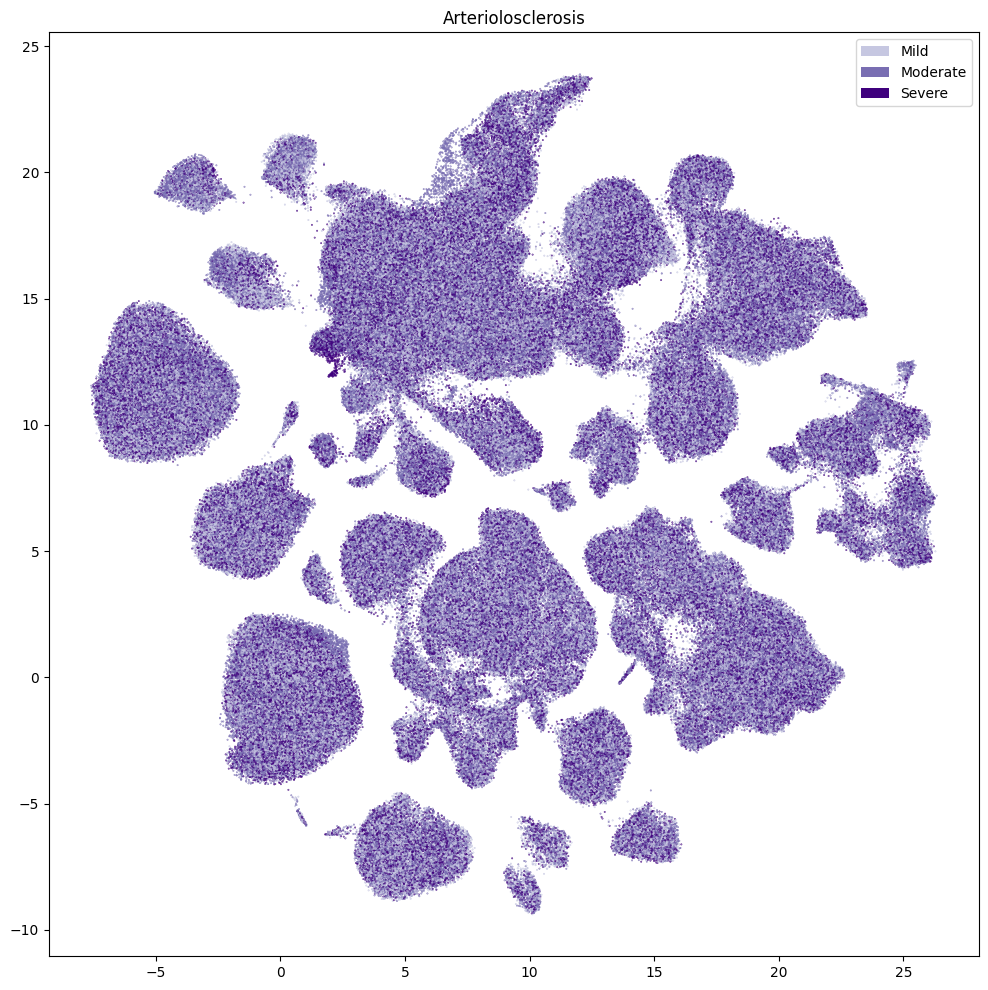
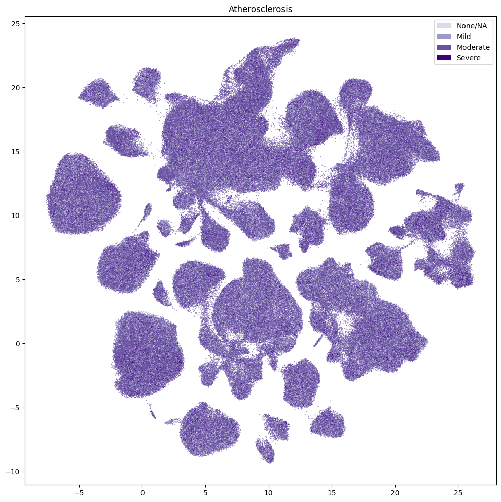
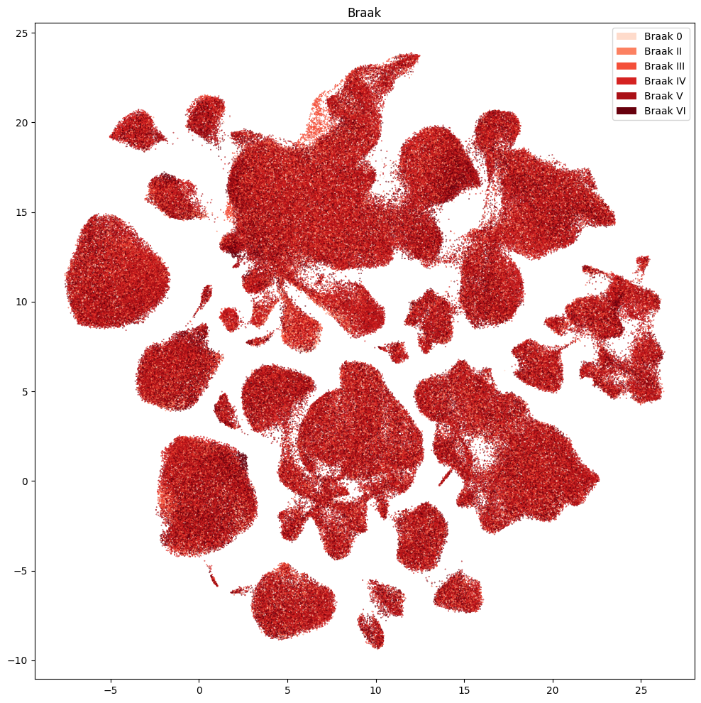
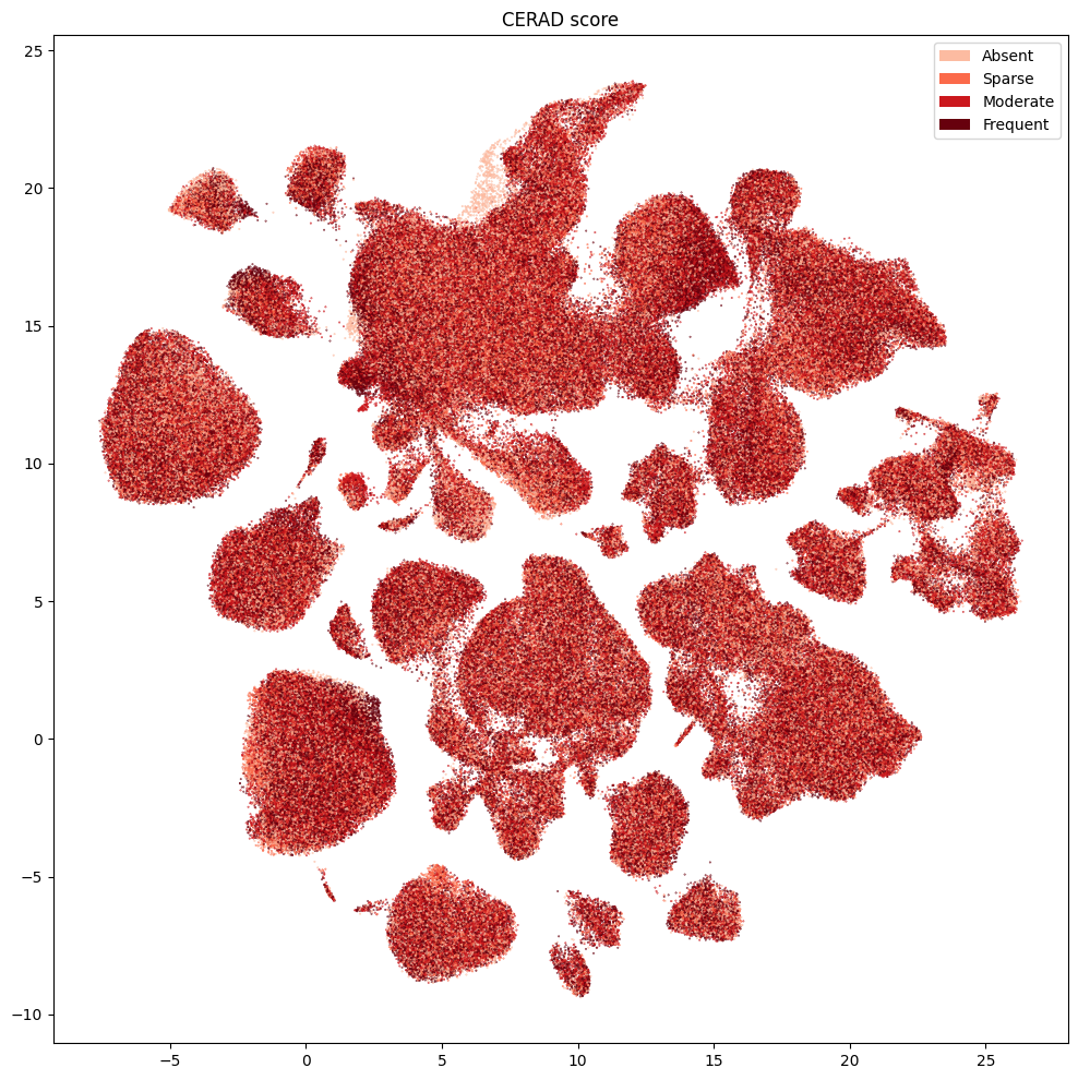
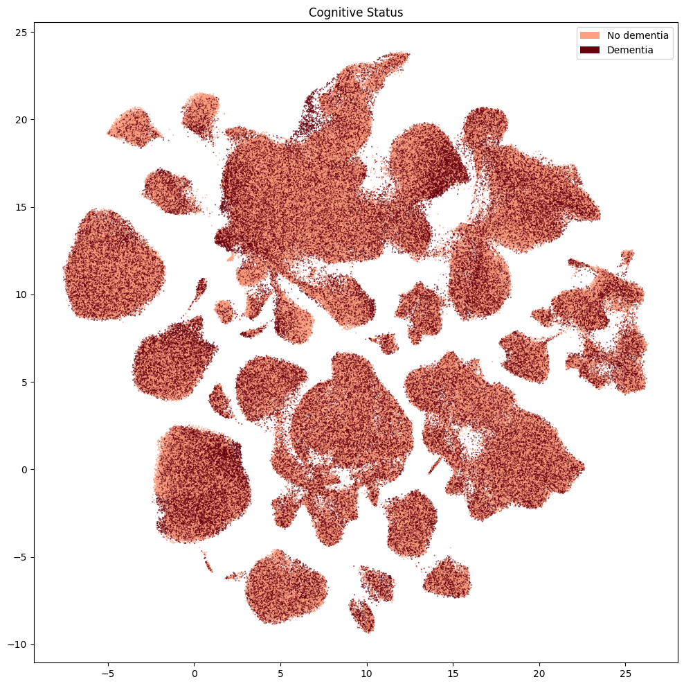
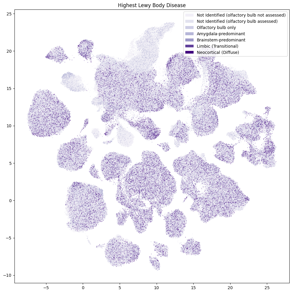
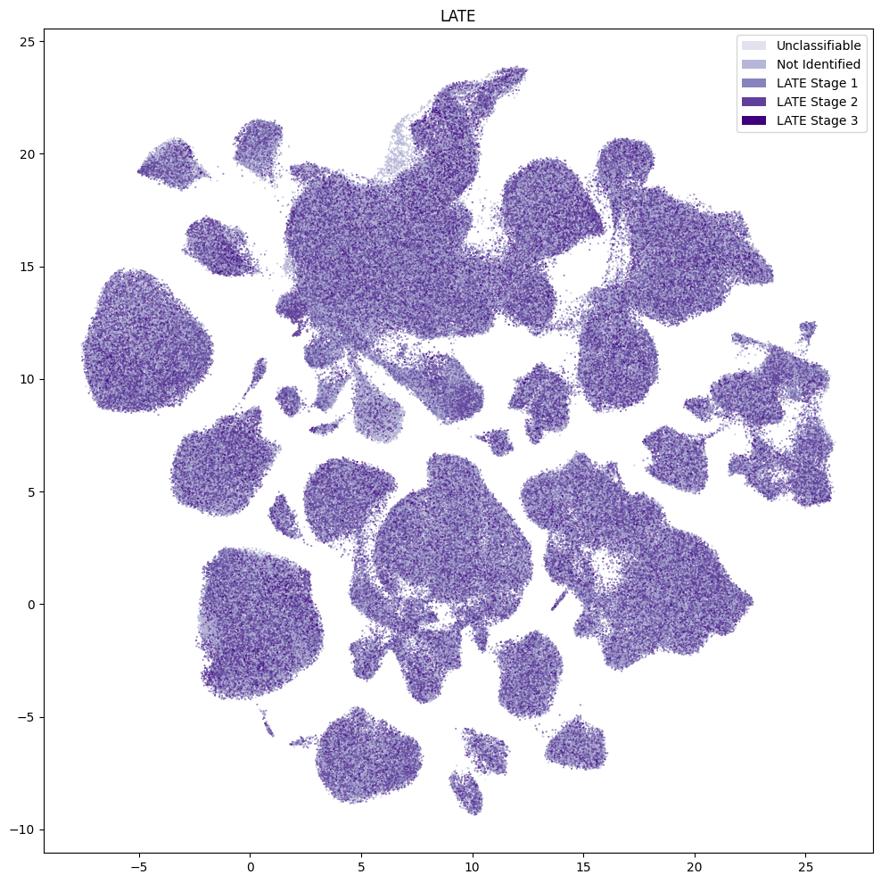
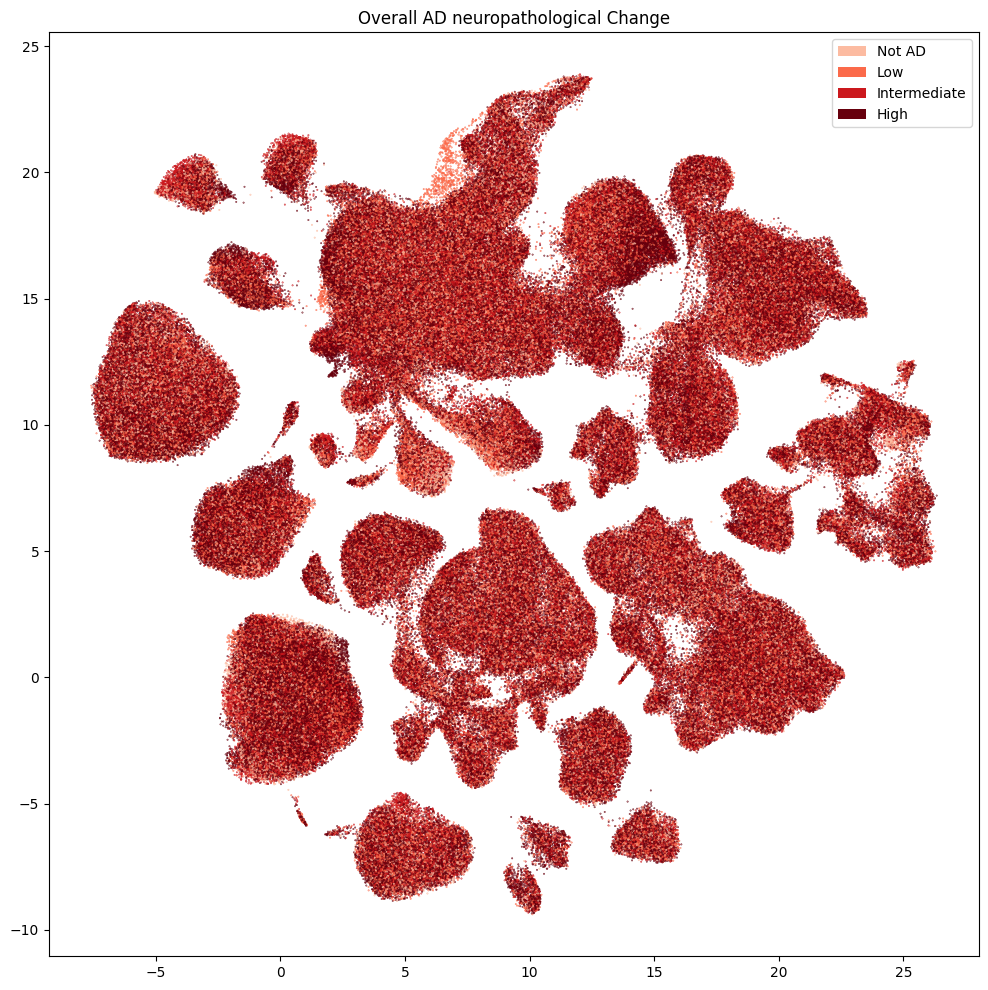
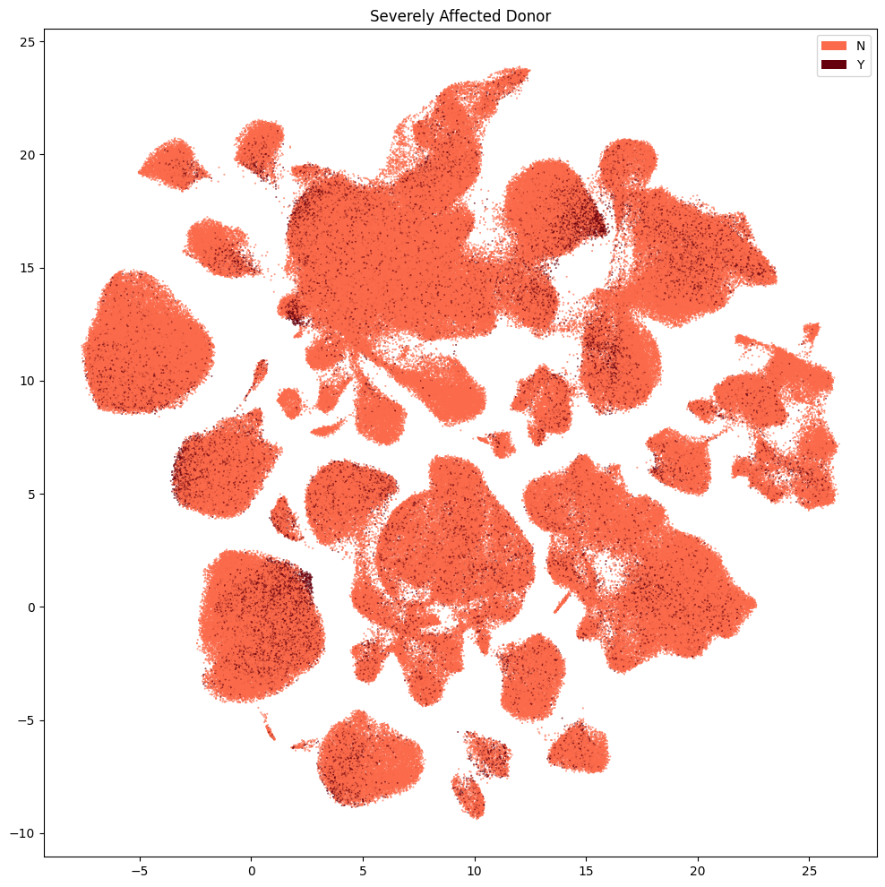
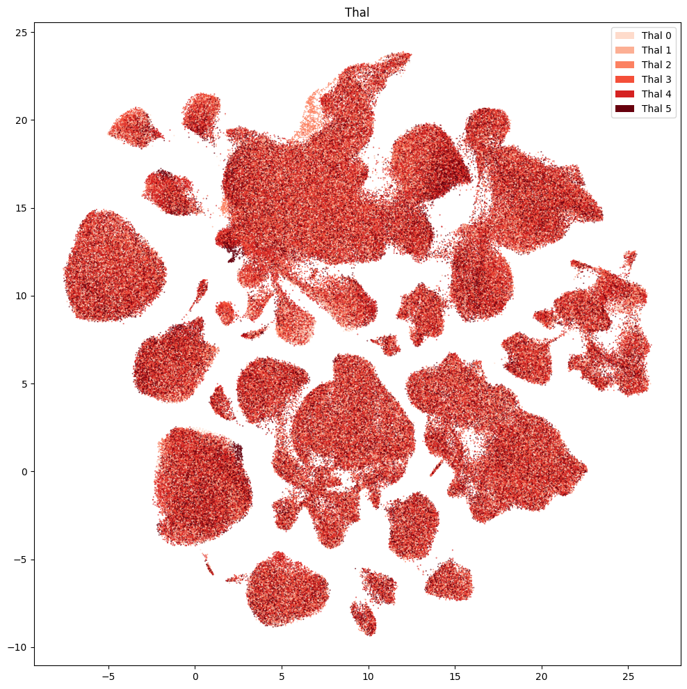
New we plot the UMAP with for the various disease markers in the data.

for disease_value in value_sets[value_sets['table'] == 'disease']['field'].unique():
    fig, ax = plot_umap(
        plot_cell_extended['x'],
        plot_cell_extended['y'],
        cc=plot_cell_extended[f'{disease_value}_color'],
        labels=plot_cell_extended[f'{disease_value}'],
        term_orders=plot_cell_extended[f'{disease_value}_order'],
        fig_width=12,
        fig_height=12
    )
    res = ax.set_title(f"{disease_value}")
    plt.show()

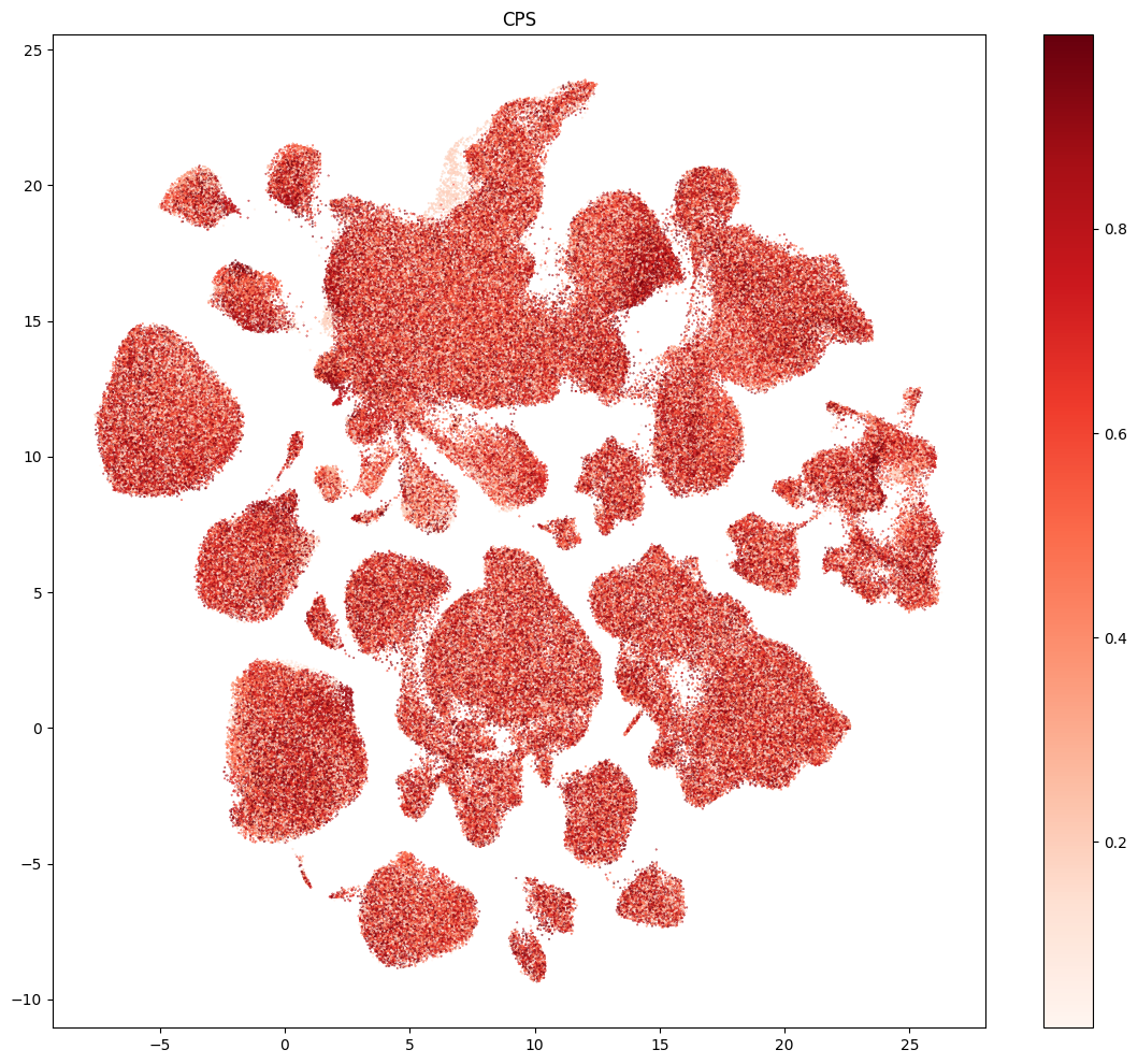
Finally, we’ll plot the pseudo-progression scores (CPS) for these data.

fig, ax = plot_umap(
    plot_cell_extended['x'],
    plot_cell_extended['y'],
    val=plot_cell_extended['CPS_Global'],
    cmap=plt.cm.Reds,
    fig_width=14,
    fig_height=12,
    colorbar=True,
)
res = ax.set_title("CPS")
plt.show()

Taxonomy Information

The final set of metadata we load into our extended cell metadata file maps the cells into their assigned cluster in the taxonomy. We additionally load metadata for the clusters and compute useful information, such as the number of cells in each taxon at each level of the taxonomy. In this notebook cluster refers to the leaf node of the taxonomy as is the case throughout abc_atlas_access. In this taxonomy, the highest granularity cell type is called ‘supertype’; therefore, when you see the term ‘cluster’ below it refers to the leaf node of the taxonomy aka, the supertypes.

First, we load information associated with the lowest level in the taxonomy. This includes a useful alias value for each cluster as well as the number of cells in each supertype.

cluster = abc_cache.get_metadata_dataframe(
    directory='SEA-AD-Multiregion-taxonomy',
    file_name='cluster',
    dtype={'number_of_cells': 'Int64'}
).rename(columns={'label': 'cluster_annotation_term_label'}).set_index('cluster_annotation_term_label')
cluster.head()

cluster.csv: 100%|██████████| 6.03k/6.03k [00:00<00:00, 72.4kMB/s]

	cluster_alias	number_of_cells
cluster_annotation_term_label
CS20260630_SUPR_001	1	88293
CS20260630_SUPR_002	2	3295
CS20260630_SUPR_003	3	2368
CS20260630_SUPR_004	4	700
CS20260630_SUPR_005	5	14450

Next, we load the table that describes the levels in the taxonomy from class at the highest to supertype at the lowest level.

cluster_annotation_term_set = abc_cache.get_metadata_dataframe(
    directory='SEA-AD-Multiregion-taxonomy',
    file_name='cluster_annotation_term_set'
).rename(columns={'label': 'cluster_annotation_term_label'})
cluster_annotation_term_set

cluster_annotation_term_set.csv: 100%|██████████| 208/208 [00:00<00:00, 2.25kMB/s]

	name	cluster_annotation_term_label	description	order	parent_term_set_label
0	Class	CCN20260630_LEVEL_0	Class	0	NaN
1	Subclass	CCN20260630_LEVEL_1	Subclass	1	CCN20260630_LEVEL_0
2	Supertype	CCN20260630_LEVEL_2	Supertype	2	CCN20260630_LEVEL_1

For the supertypes, we load information on the annotations for each supertype. This also includes the term order and color information which we will use to plot later.

cluster_annotation_term = abc_cache.get_metadata_dataframe(
    directory='SEA-AD-Multiregion-taxonomy',
    file_name='cluster_annotation_term',
).rename(columns={'label': 'cluster_annotation_term_label'}).set_index('cluster_annotation_term_label')
cluster_annotation_term

cluster_annotation_term.csv: 100%|██████████| 32.3k/32.3k [00:00<00:00, 241kMB/s]

	name	cluster_annotation_term_set_label	cluster_annotation_term_set_name	color_hex_triplet	term_order	term_set_order	parent_term_label	parent_term_name	parent_term_set_label	CCN20230508_label
cluster_annotation_term_label
CS20260630_CLAS_001	Neuronal: GABAergic	CCN20260630_LEVEL_0	Class	#F05A28	1	0	NaN	NaN	NaN	NaN
CS20260630_CLAS_002	Neuronal: Glutamatergic	CCN20260630_LEVEL_0	Class	#00ADF8	2	0	NaN	NaN	NaN	NaN
CS20260630_CLAS_003	Non-neuronal and Non-neural	CCN20260630_LEVEL_0	Class	#808080	3	0	NaN	NaN	NaN	NaN
CS20260630_SCLA_023	Astrocyte	CCN20260630_LEVEL_1	Subclass	#665C47	23	1	CS20260630_CLAS_003	Non-neuronal and Non-neural	CCN20260630_LEVEL_0	NaN
CS20260630_SCLA_021	CA2-4	CCN20260630_LEVEL_1	Subclass	#D5BF41	21	1	CS20260630_CLAS_002	Neuronal: Glutamatergic	CCN20260630_LEVEL_0	NaN
...	...	...	...	...	...	...	...	...	...	...
CS20260630_SUPR_038	Vip_25-SEAAD	CCN20260630_LEVEL_2	Supertype	#492C56	38	2	CS20260630_SCLA_005	Vip	CCN20260630_LEVEL_1	NaN
CS20260630_SUPR_039	Vip_4	CCN20260630_LEVEL_2	Supertype	#D0AEDC	39	2	CS20260630_SCLA_005	Vip	CCN20260630_LEVEL_1	CS20230508_SUPT_0022
CS20260630_SUPR_040	Vip_5	CCN20260630_LEVEL_2	Supertype	#C7A5D3	40	2	CS20260630_SCLA_005	Vip	CCN20260630_LEVEL_1	CS20230508_SUPT_0023
CS20260630_SUPR_041	Vip_6	CCN20260630_LEVEL_2	Supertype	#BE9DCA	41	2	CS20260630_SCLA_005	Vip	CCN20260630_LEVEL_1	CS20230508_SUPT_0024
CS20260630_SUPR_042	Vip_9	CCN20260630_LEVEL_2	Supertype	#B494C1	42	2	CS20260630_SCLA_005	Vip	CCN20260630_LEVEL_1	CS20230508_SUPT_0025

239 rows × 10 columns

Finally, we load the cluster to cluster annotation membership table. Each row in this table is a mapping between the supertypes and every level of the taxonomy it belongs to, including itself. We’ll use this table in a groupby to allow us to count up the number of clusters at each taxonomy level and sum the number of cells in each taxon in the taxonomy a all levels.

cluster_to_cluster_annotation_membership = abc_cache.get_metadata_dataframe(
    directory='SEA-AD-Multiregion-taxonomy',
    file_name='cluster_to_cluster_annotation_membership'
).set_index('cluster_annotation_term_label')
membership_with_cluster_info = cluster_to_cluster_annotation_membership.join(
    cluster.reset_index().set_index('cluster_alias')[['number_of_cells']],
    on='cluster_alias'
)
membership_with_cluster_info = membership_with_cluster_info.join(cluster_annotation_term, rsuffix='_anno_term').reset_index()
membership_groupby = membership_with_cluster_info.groupby(
    ['cluster_alias', 'cluster_annotation_term_set_name']
)
membership_with_cluster_info.head()

cluster_to_cluster_annotation_membership.csv: 100%|██████████| 40.6k/40.6k [00:00<00:00, 334kMB/s]

	cluster_annotation_term_label	cluster_annotation_term_set_name	cluster_annotation_term_name	cluster_alias	cluster_annotation_term_set_label	number_of_cells	name	cluster_annotation_term_set_label_anno_term	cluster_annotation_term_set_name_anno_term	color_hex_triplet	term_order	term_set_order	parent_term_label	parent_term_name	parent_term_set_label	CCN20230508_label
0	CS20260630_CLAS_001	Class	Neuronal: GABAergic	1	CCN20260630_LEVEL_0	88293	Neuronal: GABAergic	CCN20260630_LEVEL_0	Class	#F05A28	1	0	NaN	NaN	NaN	NaN
1	CS20260630_CLAS_001	Class	Neuronal: GABAergic	2	CCN20260630_LEVEL_0	3295	Neuronal: GABAergic	CCN20260630_LEVEL_0	Class	#F05A28	1	0	NaN	NaN	NaN	NaN
2	CS20260630_CLAS_001	Class	Neuronal: GABAergic	3	CCN20260630_LEVEL_0	2368	Neuronal: GABAergic	CCN20260630_LEVEL_0	Class	#F05A28	1	0	NaN	NaN	NaN	NaN
3	CS20260630_CLAS_001	Class	Neuronal: GABAergic	4	CCN20260630_LEVEL_0	700	Neuronal: GABAergic	CCN20260630_LEVEL_0	Class	#F05A28	1	0	NaN	NaN	NaN	NaN
4	CS20260630_CLAS_001	Class	Neuronal: GABAergic	5	CCN20260630_LEVEL_0	14450	Neuronal: GABAergic	CCN20260630_LEVEL_0	Class	#F05A28	1	0	NaN	NaN	NaN	NaN

From the membership table, we create three tables via a groupby. First the name of each cluster and its parents.

# term_sets = abc_cache.get_metadata_dataframe(directory='WHB-taxonomy', file_name='cluster_annotation_term_set').set_index('label')
cluster_details = membership_groupby['cluster_annotation_term_name'].first().unstack()
cluster_details = cluster_details[cluster_annotation_term_set['name']] # order columns
cluster_details.fillna('Other', inplace=True)
cluster_details.head()

cluster_annotation_term_set_name	Class	Subclass	Supertype
cluster_alias
1	Neuronal: GABAergic	Lamp5 Lhx6	Lamp5_Lhx6_1
2	Neuronal: GABAergic	Lamp5 Lhx6	Lamp5_Lhx6_2-SEAAD
3	Neuronal: GABAergic	Lamp5 Lhx6	Lamp5_Lhx6_3-SEAAD
4	Neuronal: GABAergic	Lamp5 Lhx6	Lamp5_Lhx6_4-SEAAD
5	Neuronal: GABAergic	Lamp5	Lamp5_1

Next the plotting order of each of the taxons and their parents.

cluster_order = membership_groupby['term_order'].first().unstack()
cluster_order.head()

cluster_annotation_term_set_name	Class	Subclass	Supertype
cluster_alias
1	1	1	1
2	1	1	2
3	1	1	3
4	1	1	4
5	1	2	5

Finally, the colors we will use to plot for each of the unique taxons at all levels.

cluster_colors = membership_groupby['color_hex_triplet'].first().unstack()
cluster_colors = cluster_colors[cluster_annotation_term_set['name']]
cluster_colors.head()

cluster_annotation_term_set_name	Class	Subclass	Supertype
cluster_alias
1	#F05A28	#935F50	#C6A299
2	#F05A28	#935F50	#A68880
3	#F05A28	#935F50	#866E67
4	#F05A28	#935F50	#67544F
5	#F05A28	#DA808C	#F9B7C3

Next, we bring it all together by loading the mapping of cells to supertype and join into our final metadata table.

cell_to_cluster_membership = abc_cache.get_metadata_dataframe(
    directory='SEA-AD-Multiregion-taxonomy',
    file_name='cell_to_cluster_membership',
).set_index('cell_label')
cell_to_cluster_membership.head()

cell_to_cluster_membership.csv: 100%|██████████| 295M/295M [00:25<00:00, 11.8MMB/s]    

	cluster_alias	label
cell_label
AAACAGCCACTGGCTG-2001_A08	84	CS20260630_SUPR_084
AAACAGCCAGGTTATT-2001_A08	180	CS20260630_SUPR_180
AAACAGCCATTCCTCG-2001_A08	113	CS20260630_SUPR_113
AAACATGCAATGCCTA-2001_A08	80	CS20260630_SUPR_080
AAACATGCACCTCACC-2001_A08	76	CS20260630_SUPR_076

We merge this table with information from our taxons. Again, we’ll subset the full set of cells for ease of plotting.

cell_extended = cell_extended.join(cell_to_cluster_membership, rsuffix='_cell_to_cluster_membership', how='inner')
cell_extended = cell_extended.join(cluster_details, on='cluster_alias')
cell_extended = cell_extended.join(cluster_colors, on='cluster_alias', rsuffix='_color')
cell_extended = cell_extended.join(cluster_order, on='cluster_alias', rsuffix='_order')
plot_cell_extended = cell_extended[::10]

del cell_to_cluster_membership

cell_extended.head()

	cell_barcode	barcoded_cell_sample_label	library_label	alignment_job_id	doublet_score	umi_count	donor_label	exp_component_name	feature_matrix_label	dataset_label	...	label	Class	Subclass	Supertype	Class_color	Subclass_color	Supertype_color	Class_order	Subclass_order	Supertype_order
cell_label
CAATTTCAGCCTTTGA-1580_C01	CAATTTCAGCCTTTGA	1580_C01	L8HX_230126_02_E07	1244668541	0.100000	24846.0	H20.33.040	CAATTTCAGCCTTTGA-L8HX_230126_02_E07-1244668541	STG-10X	SEA-AD-Multiregion-10X	...	CS20260630_SUPR_025	Neuronal: GABAergic	Vip	Vip_1	#F05A28	#A45FBF	#E2C0EE	1	5	25
AGGTGTTGTGGTTTGT-633_F06	AGGTGTTGTGGTTTGT	633_F06	L8TX_210506_01_E08	1153814230	0.060000	7716.0	H21.33.022	AGGTGTTGTGGTTTGT-L8TX_210506_01_E08-1153814230	MTG-10X	SEA-AD-Multiregion-10X	...	CS20260630_SUPR_036	Neuronal: GABAergic	Vip	Vip_23	#F05A28	#A45FBF	#5A3D67	1	5	36
AATGCCAGTTCAAGGG-1725_C01	AATGCCAGTTCAAGGG	1725_C01	L8HX_230601_22_D04	1277848644	0.060000	32147.0	H19.33.004	AATGCCAGTTCAAGGG-L8HX_230601_22_D04-1277848644	ITG-10X	SEA-AD-Multiregion-10X	...	CS20260630_SUPR_092	Neuronal: Glutamatergic	L2/3 IT	L2/3 IT_6	#00ADF8	#B1EC30	#B0BF64	2	10	92
TACCTCGGTCAAAGAT-733_G01	TACCTCGGTCAAAGAT	733_G01	L8TX_210722_01_B08	1153814305	0.020833	10344.0	H21.33.033	TACCTCGGTCAAAGAT-L8TX_210722_01_B08-1153814305	MTG-10X	SEA-AD-Multiregion-10X	...	CS20260630_SUPR_084	Neuronal: Glutamatergic	L2/3 IT	L2/3 IT_1	#00ADF8	#B1EC30	#EEF987	2	10	84
GCACGGTTCTTCGTGC-763_H06	GCACGGTTCTTCGTGC	763_H06	L8TX_210805_01_E02	1124416548	0.312500	59494.0	H20.33.020	GCACGGTTCTTCGTGC-L8TX_210805_01_E02-1124416548	DFC-10X	SEA-AD-Multiregion-10X	...	CS20260630_SUPR_041	Neuronal: GABAergic	Vip	Vip_6	#F05A28	#A45FBF	#BE9DCA	1	5	41

5 rows × 107 columns

print_column_info(cell_extended)

Number of unique cell_barcode = 3264931 
Number of unique barcoded_cell_sample_label = 907 
Number of unique library_label = 907 
Number of unique alignment_job_id = 912 
Number of unique doublet_score = 2395 
Number of unique umi_count = 164013 
Number of unique donor_label = 84 
Number of unique exp_component_name = 6013346 
Number of unique feature_matrix_label = 10 ['AnG-10X', 'DFC-10X', 'FI-10X', 'HIP-10X', 'ITG-10X', 'LEC-10X', 'MEC-10X', 'MTG-10X', 'STG-10X', 'V1C-10X']
Number of unique dataset_label = 1 ['SEA-AD-Multiregion-10X']
Number of unique donor_species = 1 ['NCBITaxon:9606']
Number of unique species_scientific_name = 1 ['Homo sapiens']
Number of unique species_genus = 1 ['Human']
Number of unique donor_sex = 2 ['Female', 'Male']
Number of unique donor_gender = 2 ['Female', 'Male']
Number of unique donor_age = 29 ['100+ yrs', '65 yrs', '68 yrs', '69 yrs', '70 yrs', '72 yrs', '75 yrs', '77 yrs', '78 yrs', '80 yrs', '81 yrs', '82 yrs', '83 yrs', '84 yrs', '85 yrs', '86 yrs', '87 yrs', '88 yrs', '89 yrs', '90 yrs', '91 yrs', '92 yrs', '93 yrs', '94 yrs', '95 yrs', '96 yrs', '97 yrs', '98 yrs', '99 yrs']
Number of unique donor_age_value = 29 [65, 68, 69, 70, 72, 75, 77, 78, 80, 81, 82, 83, 84, 85, 86, 87, 88, 89, 90, 91, 92, 93, 94, 95, 96, 97, 98, 99, 100]
Number of unique donor_age_unit = 2 ['+ yrs_not_in_mapping', 'years']
Number of unique Race (choice=White) = 2 ['Checked', 'Unchecked']
Number of unique Race (choice=Black/ African American) = 1 ['Unchecked']
Number of unique Race (choice=Asian) = 2 ['Checked', 'Unchecked']
Number of unique Race (choice=American Indian/ Alaska Native) = 2 ['Checked', 'Unchecked']
Number of unique Race (choice=Native Hawaiian or Pacific Islander) = 1 ['Unchecked']
Number of unique Race (choice=Unknown or unreported) = 1 ['Unchecked']
Number of unique Race (choice=Other) = 2 ['Checked', 'Unchecked']
Number of unique Hispanic/Latino = 3 ['No', 'Unknown', 'Yes']
Number of unique specify other race = 1 ['Mixed']
Number of unique Highest level of education = 5 ['Bachelors', 'Graduate (PhD/Masters)', 'High School', 'Professional', 'Trade School/ Tech School']
Number of unique Years of education = 10 [12, 13, 14, 15, 16, 17, 18, 19, 20, 21]
Number of unique PMI = 60 
Number of unique Fresh Brain Weight = 74 
Number of unique Brain pH = 14 [4.5, 6.0, 6.2, 6.4, 6.5, 6.6, 6.7, 6.8, 6.9, 7.0, 7.2, 7.3, 7.4, 7.6]
Number of unique Primary Study Name = 2 ['ACT', 'ADRC Clinical Core']
Number of unique donor_race = 4 ['American Indian/Alaska Native/White/Other', 'Asian', 'White', 'White/Other']
Number of unique library_method = 3 ['10xMultiome;GEX', '10xV3.1', '10xV3.1_HT']
Number of unique barcoded_cell_sample_label_library_table = 907 
Number of unique enrichment_population = 21 ['100% NeuN+', '38% NeuN+, 62% NeuN-', '40% NeuN+, 60% NeuN-', '44% NeuN+, 56% NeuN-', '46% NeuN+, 54% NeuN-', '50% NeuN+, 50% NeuN-', '56% NeuN+, 44% NeuN-', '57% NeuN+, 43% NeuN-', '60% NeuN+, 40% NeuN-', '62% NeuN+, 38% NeuN-', '63% NeuN+, 37% NeuN-', '64% NeuN+, 36% NeuN-', '65% NeuN+, 35% NeuN-', '66% NeuN+, 34% NeuN-', '68% NeuN+, 32% NeuN-', '70% NeuN +, 30% NeuN-', '70% NeuN+, 30% NeuN-', '71% NeuN+, 29% NeuN-', '74% NeuN+, 26% NeuN-', '90% NeuN+, 10% NeuN-', 'NeuN-positive and NeuN-negative']
Number of unique cell_specimen_type = 1 ['Nuclei']
Number of unique region_of_interest_label = 10 ['AnG', 'DFC', 'FI', 'HIP', 'ITG', 'LEC', 'MEC', 'MTG', 'STG', 'V1C']
Number of unique region_of_interest_name = 10 ['angular gyrus', 'dorsolateral prefrontal cortex', 'frontal agranular insular cortex (area FI)', 'hippocampus (hippocampal formation)', 'inferior temporal gyrus', 'lateral (anterior) entorhinal cortex', 'medial (posterior) entorhinal cortex', 'middle temporal gyrus', 'primary visual cortex (striate cortex, area V1/17)', 'superior temporal gyrus']
Number of unique parcellation_term_identifier = 10 ['DHBA:10173', 'DHBA:10269', 'DHBA:10294', 'DHBA:10318', 'DHBA:10319', 'DHBA:10329', 'DHBA:12136', 'DHBA:12140', 'DHBA:12141', 'DHBA:12142']
Number of unique Brain Region = 10 ['AnG', 'DFC', 'FI', 'HIP', 'ITG', 'LEC', 'MEC', 'MTG', 'STG', 'V1C']
Number of unique donor_label_library_table = 84 
Number of unique Overall AD neuropathological Change = 4 ['High', 'Intermediate', 'Low', 'Not AD']
Number of unique Thal = 6 ['Thal 0', 'Thal 1', 'Thal 2', 'Thal 3', 'Thal 4', 'Thal 5']
Number of unique Braak = 6 ['Braak 0', 'Braak II', 'Braak III', 'Braak IV', 'Braak V', 'Braak VI']
Number of unique CERAD score = 4 ['Absent', 'Frequent', 'Moderate', 'Sparse']
Number of unique Overall CAA Score = 4 ['Mild', 'Moderate', 'Not identified', 'Severe']
Number of unique Highest Lewy Body Disease = 7 ['Amygdala-predominant', 'Brainstem-predominant', 'Limbic (Transitional)', 'Neocortical (Diffuse)', 'Not Identified (olfactory bulb assessed)', 'Not Identified (olfactory bulb not assessed)', 'Olfactory bulb only']
Number of unique Total Microinfarcts (not observed grossly) = 10 [0, 1, 2, 3, 4, 5, 7, 9, 11, 15]
Number of unique Total microinfarcts in screening sections = 9 [0, 1, 2, 3, 4, 5, 8, 9, 10]
Number of unique Atherosclerosis = 4 ['Mild', 'Moderate', 'None/NA', 'Severe']
Number of unique Arteriolosclerosis = 3 ['Mild', 'Moderate', 'Severe']
Number of unique LATE = 5 ['LATE Stage 1', 'LATE Stage 2', 'LATE Stage 3', 'Not Identified', 'Unclassifiable']
Number of unique Cognitive Status = 2 ['Dementia', 'No dementia']
Number of unique Last CASI Score = 29 [66.0, 67.0, 68.0, 70.0, 71.0, 74.0, 75.0, 77.0, 78.0, 79.0, 80.0, 81.0, 83.0, 84.0, 85.0, 86.0, 87.0, 88.0, 89.0, 90.0, 91.0, 92.0, 93.0, 94.0, 95.0, 96.0, 97.0, 98.0, 99.0]
Number of unique Interval from last CASI in months = 60 
Number of unique Last MMSE Score = 18 [6.0, 11.0, 14.0, 17.0, 18.0, 19.0, 20.0, 21.0, 22.0, 23.0, 24.0, 25.0, 26.0, 27.0, 28.0, 29.0, 30.0, 33.0]
Number of unique Interval from last MMSE in months = 70 
Number of unique Last MOCA Score = 10 [4.0, 7.0, 14.0, 16.0, 17.0, 19.0, 20.0, 21.0, 23.0, 25.0]
Number of unique Interval from last MOCA in months = 14 [10.1, 11.1, 14.9, 15.2, 15.8, 22.1, 23.9, 33.4, 36.1, 39.5, 41.2, 45.1, 51.3, 62.2]
Number of unique APOE Genotype = 6 ['2/2', '2/3', '2/4', '3/3', '3/4', '4/4']
Number of unique Severely Affected Donor = 2 ['N', 'Y']
Number of unique CPS_Global = 84 
Number of unique region_of_interest_label_color = 10 ['#00008b', '#006400', '#008080', '#00bfff', '#32cd32', '#9932cc', '#9acd32', '#b22222', '#ff0000', '#ff8c00']
Number of unique region_of_interest_label_order = 10 [1, 3, 4, 5, 6, 7, 8, 9, 10, 11]
Number of unique APOE Genotype_color = 6 ['#67000d', '#b21218', '#e32f27', '#fb6a4a', '#fca082', '#fdd4c2']
Number of unique APOE Genotype_order = 6 [1, 2, 3, 4, 5, 6]
Number of unique Arteriolosclerosis_color = 3 ['#3f007d', '#796eb2', '#c6c7e1']
Number of unique Arteriolosclerosis_order = 3 [1, 2, 3]
Number of unique Atherosclerosis_color = 4 ['#3f007d', '#6a51a3', '#9e9ac8', '#dadaeb']
Number of unique Atherosclerosis_order = 4 [1, 2, 3, 4]
Number of unique Braak_color = 6 ['#67000d', '#aa1016', '#d52221', '#f44f39', '#fc8161', '#fedbcb']
Number of unique Braak_order = 6 [1, 3, 4, 5, 6, 7]
Number of unique CERAD score_color = 4 ['#67000d', '#cb181d', '#fb6a4a', '#fcbba1']
Number of unique CERAD score_order = 4 [1, 2, 3, 4]
Number of unique Cognitive Status_color = 2 ['#67000d', '#fca082']
Number of unique Cognitive Status_order = 2 [1, 3]
Number of unique LATE_color = 5 ['#3f007d', '#61409b', '#8683bd', '#b6b6d8', '#e2e2ef']
Number of unique LATE_order = 5 [1, 2, 3, 4, 5]
Number of unique Highest Lewy Body Disease_color = 7 ['#3f007d', '#61409b', '#9e9ac8', '#b6b6d8', '#cecee5', '#e2e2ef', '#f2f0f7']
Number of unique Highest Lewy Body Disease_order = 7 [1, 2, 3, 4, 5, 8, 10]
Number of unique Overall AD neuropathological Change_color = 4 ['#67000d', '#cb181d', '#fb6a4a', '#fcbba1']
Number of unique Overall AD neuropathological Change_order = 4 [1, 2, 3, 4]
Number of unique Severely Affected Donor_color = 2 ['#67000d', '#fb6a4a']
Number of unique Severely Affected Donor_order = 2 [1, 2]
Number of unique Thal_color = 6 ['#67000d', '#d52221', '#f44f39', '#fc8161', '#fcaf94', '#fedbcb']
Number of unique Thal_order = 6 [1, 2, 3, 4, 5, 7]
Number of unique donor_sex_color = 2 ['#565353', '#ADC4C3']
Number of unique donor_sex_order = 2 [1, 2]
Number of unique donor_gender_color = 2 ['#565353', '#ADC4C3']
Number of unique donor_gender_order = 2 [1, 2]
Number of unique donor_race_color = 4 ['#19d79d', '#bc6b63', '#e6fd9a', '#f7f184']
Number of unique donor_race_order = 4 [64, 65, 125, 126]
Number of unique x = 5550464 
Number of unique y = 5397802 
Number of unique cluster_alias = 207 
Number of unique label = 207 
Number of unique Class = 3 ['Neuronal: GABAergic', 'Neuronal: Glutamatergic', 'Non-neuronal and Non-neural']
Number of unique Subclass = 29 ['Astrocyte', 'CA2-4', 'Chandelier', 'DG', 'EC IT', 'Endothelial', 'Ependymal', 'Immune', 'L2/3 IT', 'L4 IT', 'L5 ET', 'L5 IT', 'L5/6 NP', 'L6 CT', 'L6 IT', 'L6 IT Car3', 'L6b', 'Lamp5', 'Lamp5 Lhx6', 'OPC', 'Oligodendrocyte', 'Pax6', 'Pvalb', 'Sncg', 'Sst', 'Sst Chodl', 'Sub-CA1', 'VLMC & Perivascular', 'Vip']
Number of unique Supertype = 207 
Number of unique Class_color = 3 ['#00ADF8', '#808080', '#F05A28']
Number of unique Subclass_color = 29 ['#00E5E5', '#0D5B78', '#2D8CB8', '#374A45', '#3E9E64', '#50B2AD', '#5100FF', '#53776C', '#665C47', '#697255', '#7044AA', '#71238C', '#73BC48', '#7A5151', '#8D6C62', '#935F50', '#94AF97', '#A19922', '#A45FBF', '#B1B10C', '#B1EC30', '#D5BF41', '#D8442B', '#D93137', '#DA808C', '#DECB54', '#DF70FF', '#F641A8', '#FF9900']
Number of unique Supertype_color = 207 
Number of unique Class_order = 3 [1, 2, 3]
Number of unique Subclass_order = 29 [1, 2, 3, 4, 5, 6, 7, 8, 9, 10, 11, 12, 13, 14, 15, 16, 17, 18, 19, 20, 21, 22, 23, 24, 25, 26, 27, 28, 29]
Number of unique Supertype_order = 207 

Plotting the taxonomy

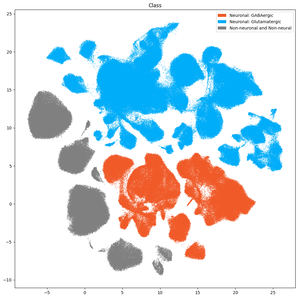
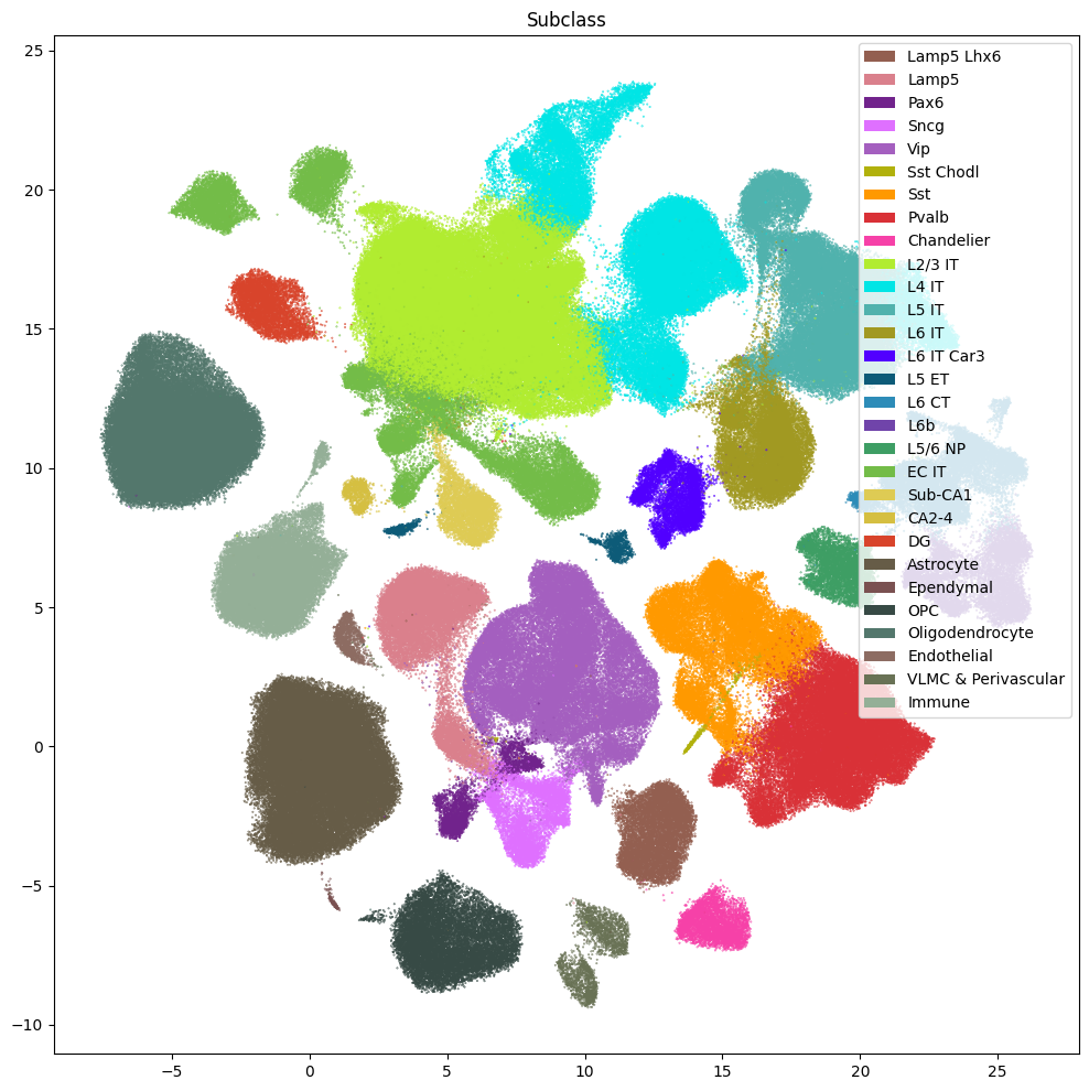
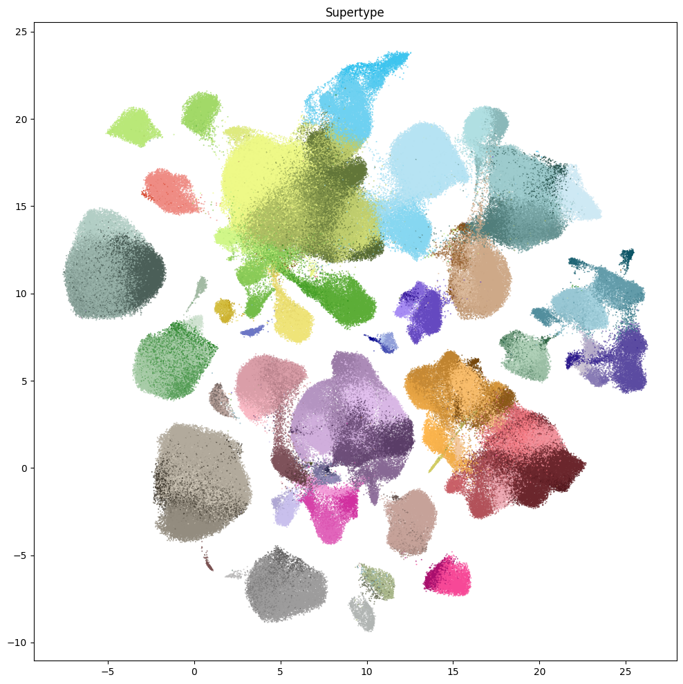
Now that we have our cells with associated taxonomy information, we’ll plot them into the UMAP we showed previously.

Below we plot the taxonomy mapping of the cells for each level in the taxonomy.

fig, ax = plot_umap(
    plot_cell_extended['x'],
    plot_cell_extended['y'],
    cc=plot_cell_extended['Class_color'],
    labels=plot_cell_extended['Class'],
    term_orders=plot_cell_extended['Class_order'],
    fig_width=12,
    fig_height=12
)
res = ax.set_title("Class")
plt.show()

fig, ax = plot_umap(
    plot_cell_extended['x'],
    plot_cell_extended['y'],
    cc=plot_cell_extended['Subclass_color'],
    labels=plot_cell_extended['Subclass'],
    term_orders=plot_cell_extended['Subclass_order'],
    fig_width=12,
    fig_height=12
)
res = ax.set_title("Subclass")
plt.show()

fig, ax = plot_umap(
    plot_cell_extended['x'],
    plot_cell_extended['y'],
    cc=plot_cell_extended['Supertype_color'],
    fig_width=12,
    fig_height=12
)
res = ax.set_title("Supertype")
plt.show()

Below we plot the Subclass level of the taxonomy against paired with a plot Brain Regions in the UMAP.

fig, ax = plt.subplots(1, 2)
fig.set_size_inches(18, 9)
ax = ax.flatten()
term_to_plot_1 = 'region_of_interest_label'
plot_umap(
    cell_extended['x'][::10],
    cell_extended['y'][::10],
    cc=cell_extended[term_to_plot_1 + '_color'][::10],
    labels=cell_extended[term_to_plot_1][::10],
    term_orders=cell_extended[term_to_plot_1 + '_order'][::10],
    fig=fig,
    ax=ax[0],
)
ax[0].set_title('Brain Region')
term_to_plot_2 = 'Subclass'
plot_umap(
    cell_extended['x'][::10],
    cell_extended['y'][::10],
    cc=cell_extended[term_to_plot_2 + '_color'][::10],
    labels=cell_extended[term_to_plot_2][::10],
    term_orders=cell_extended[term_to_plot_2 + '_order'][::10],
    fig=fig,
    ax=ax[1],
)
ax[1].set_title(f'Subclass')
plt.tight_layout()
plt.show()

Aggregating supertype and cells counts.

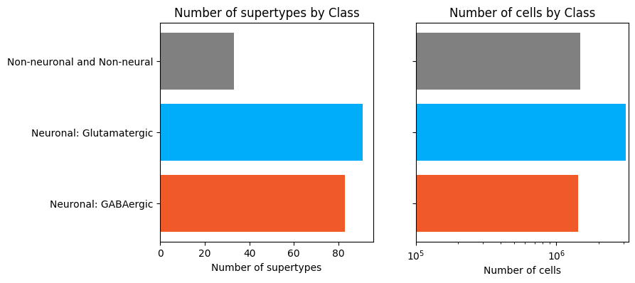
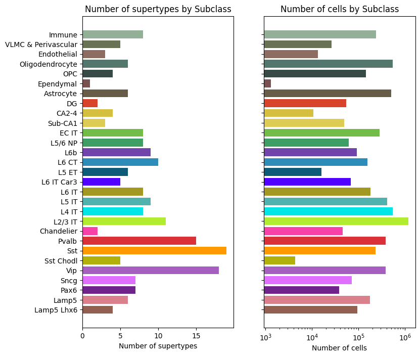
Let’s investigate the taxonomy information a bit more. In this section, we’ll create bar plots showing the number of supertypes and cells at each level in the taxonomy.

First, we need to compute the number of supertype that are in each of the cell type taxons above it. This is accomplished by a simple groupby in Pandas.

term_cluster_count = membership_with_cluster_info.reset_index().groupby(
        ['cluster_annotation_term_label']
    )[['cluster_alias']].count()
term_cluster_count.columns = ['number_of_supertypes']
term_cluster_count.head()

	number_of_supertypes
cluster_annotation_term_label
CS20260630_CLAS_001	83
CS20260630_CLAS_002	91
CS20260630_CLAS_003	33
CS20260630_SCLA_001	4
CS20260630_SCLA_002	6

term_cell_count = membership_with_cluster_info.reset_index().groupby(
    ['cluster_annotation_term_label']
)[['number_of_cells']].sum()
term_cell_count.head()

	number_of_cells
cluster_annotation_term_label
CS20260630_CLAS_001	1421338
CS20260630_CLAS_002	3110538
CS20260630_CLAS_003	1481470
CS20260630_SCLA_001	94656
CS20260630_SCLA_002	175755

# Join counts with the term dataframe
term_with_counts = cluster_annotation_term.join(term_cluster_count)
term_with_counts = term_with_counts.join(term_cell_count)
term_with_counts.head()

	name	cluster_annotation_term_set_label	cluster_annotation_term_set_name	color_hex_triplet	term_order	term_set_order	parent_term_label	parent_term_name	parent_term_set_label	CCN20230508_label	number_of_supertypes	number_of_cells
cluster_annotation_term_label
CS20260630_CLAS_001	Neuronal: GABAergic	CCN20260630_LEVEL_0	Class	#F05A28	1	0	NaN	NaN	NaN	NaN	83	1421338
CS20260630_CLAS_002	Neuronal: Glutamatergic	CCN20260630_LEVEL_0	Class	#00ADF8	2	0	NaN	NaN	NaN	NaN	91	3110538
CS20260630_CLAS_003	Non-neuronal and Non-neural	CCN20260630_LEVEL_0	Class	#808080	3	0	NaN	NaN	NaN	NaN	33	1481470
CS20260630_SCLA_023	Astrocyte	CCN20260630_LEVEL_1	Subclass	#665C47	23	1	CS20260630_CLAS_003	Non-neuronal and Non-neural	CCN20260630_LEVEL_0	NaN	6	511124
CS20260630_SCLA_021	CA2-4	CCN20260630_LEVEL_1	Subclass	#D5BF41	21	1	CS20260630_CLAS_002	Neuronal: Glutamatergic	CCN20260630_LEVEL_0	NaN	4	10572

Below we create a function to plot the supertype and cell counts in a bar graph, coloring by the associated taxon level.

def bar_plot_by_level_and_type(
        df: pd.DataFrame,
        level: str, fig_width:
        float = 8.5, fig_height:
        float = 4,
        cell_min: int = None,
        supertype_min: int = None
    ):
    """Plot the number of cells by the specified level.

    Parameters
    ----------
    df : pd.DataFrame
        DataFrame containing cluster annotation terms with counts.
    level : str
        The level of the taxonomy to plot (e.g., 'Neighborhood', 'Class', 'Subclass', 'Group', 'Cluster').
    fig_width : float, optional
        Width of the figure in inches. Default is 8.5.
    fig_height : float, optional
        Height of the figure in inches. Default is 4.
    """

    fig, ax = plt.subplots(1, 2)
    fig.set_size_inches(fig_width, fig_height)

    for idx, ctype in enumerate(['supertypes', 'cells']):

        pred = (df['cluster_annotation_term_set_name'] == level)
        sort_order = np.argsort(df[pred]['term_order'])
        names = df[pred]['name'].iloc[sort_order]
        counts = df[pred]['number_of_%s' % ctype].iloc[sort_order]
        colors = df[pred]['color_hex_triplet'].iloc[sort_order]
        
        ax[idx].barh(names, counts, color=colors)
        ax[idx].set_title('Number of %s by %s' % (ctype,level))
        ax[idx].set_xlabel('Number of %s' % ctype)
        if ctype == 'supertypes' and supertype_min is not None:
                ax[idx].set_xlim(left=supertype_min)
        if ctype == 'cells':
            if cell_min is not None:
                ax[idx].set_xlim(left=cell_min)
            ax[idx].set_xscale('log')
        
        if idx > 0:
            ax[idx].set_yticklabels([])

    return fig, ax

Now let’s plot the counts the taxonomy levels class and subclass.

fig, ax = bar_plot_by_level_and_type(term_with_counts, 'Class', cell_min=10 ** 5)
plt.show()

fig, ax = bar_plot_by_level_and_type(
    term_with_counts,
    'Subclass',
    fig_height=8
)
plt.show()

Visualizing the SEA-AD Multiregion Taxonomy

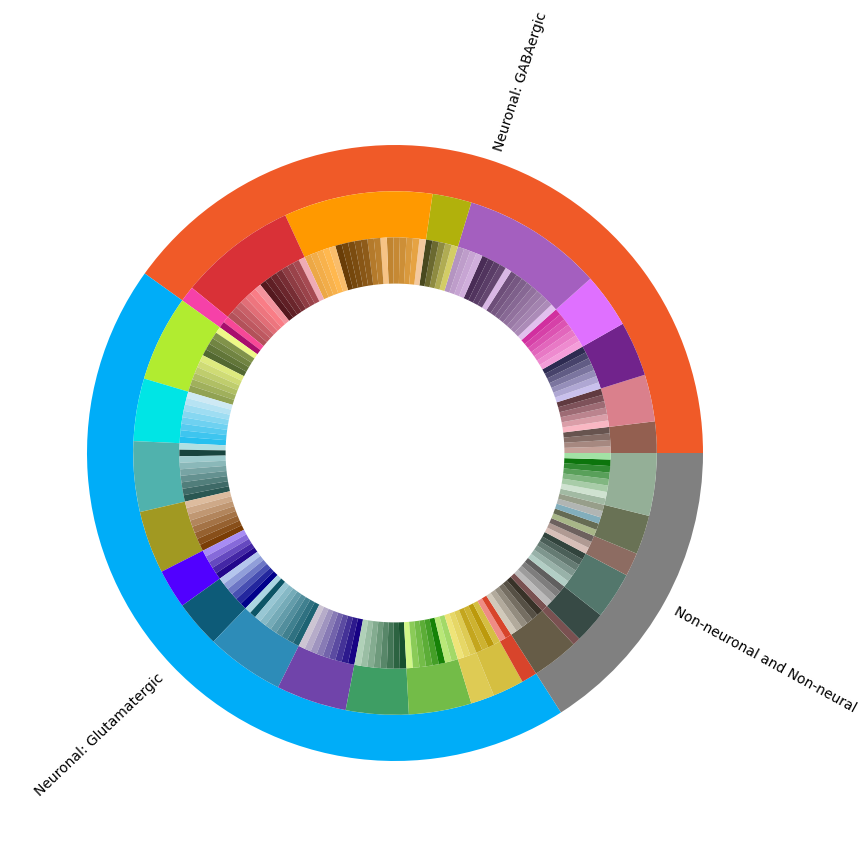
Term sets: Class, Subclass, and Supertype define the SEA-AD Multiregion taxonomy. We can visualize the taxonomy as a sunburst diagram that shows the single inheritance hierarchy through a series of rings, that are sliced for each annotation term. Each ring corresponds to a level in the hierarchy. We have ordered the rings so that the class level. Rings are divided based on their hierarchical relationship to the parent slice.

levels = ['Class', 'Subclass', 'Supertype']
df = {}

# Copy the term order of the parent into each of the level below it.
if term_with_counts.index.name != 'cluster_annotation_term_label':
    term_with_counts = term_with_counts.set_index('cluster_annotation_term_label')
term_with_counts['parent_order'] = ""
for idx, row in term_with_counts.iterrows():
    if pd.isna(row['parent_term_label']):
        continue
    term_with_counts.loc[idx, 'parent_order'] = term_with_counts.loc[row['parent_term_label']]['term_order']

term_with_counts = term_with_counts.reset_index()
for lvl in levels:
    pred = term_with_counts['cluster_annotation_term_set_name'] == lvl
    df[lvl] = term_with_counts[pred]
    df[lvl] = df[lvl].sort_values(['parent_order', 'term_order'])

fig, ax = plt.subplots()
fig.set_size_inches(10, 10)
size = 0.15

for i, lvl in enumerate(levels):
    
    if lvl == 'Class':
        ax.pie(df[lvl]['number_of_supertypes'],
               colors=df[lvl]['color_hex_triplet'],
               labels = df[lvl]['name'],
               rotatelabels=True,
               labeldistance=1.025,
               radius=1,
               wedgeprops=dict(width=size, edgecolor=None),
               startangle=0)
    else :
        ax.pie(df[lvl]['number_of_supertypes'],
               colors=df[lvl]['color_hex_triplet'],
               radius=1-i*size,
               wedgeprops=dict(width=size, edgecolor=None),
               startangle=0)
term_with_counts = term_with_counts.set_index('cluster_annotation_term_label')
plt.show()

Alzheimer’s Disease metrics

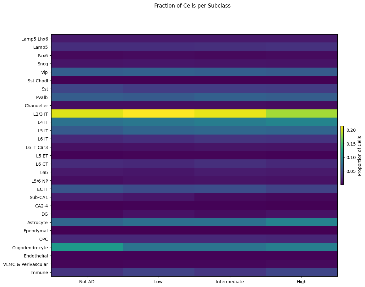
Below we show some example plots for a specific AD metric (in this case Overall AD neuropathological Change).

The function below returns a heatmap of the fraction of cells in a given pair of features (col_1, col_2) normalized by the total in number cells in the second feature given (col_2).

import matplotlib as mpl

def plot_heatmap(
    df: pd.DataFrame,
    col_1: str,
    col_2: str,
    fig_width: float = 8,
    fig_height: float = 4,
    vmax: float = None,
    cmap: plt.cm = plt.cm.magma,
    log=False
):
    """Plot a heatmap of the proportion of cells in each group defined by col_1 and col_2.

    The values in the heatmap represent the proportion of cells in each group normalized by the
    total number of cells in each column group (col_2).

    Parameters
    ----------
    df : pd.DataFrame
        DataFrame containing cell metadata and gene expression values.
    col_1 : str
        Column name in df to group by for the rows of the heatmap.
    col_2 : str
        Column name in df to group by for the columns of the heatmap.
    fig_width : float, optional
        Width of the figure in inches.
    fig_height : float, optional
        Height of the figure in inches.
    vmax : float, optional
        Maximum value for the color scale. If None, it is set to the maximum value in the data.
    cmap : matplotlib colormap, optional
        Colormap to use for the heatmap.
    log : bool, optional
        If True, the values will be log-transformed before plotting.

    Returns
    -------
    fig : matplotlib.figure.Figure
        The figure object containing the heatmap.
    ax : array of matplotlib.axes.Axes
        The axes objects for each species.
    """

    fig, ax = plt.subplots(1, 1)
    fig.set_size_inches(fig_width, fig_height)

    grouped = df.groupby([col_1, col_2])['cell_barcode'].count().unstack()
    grouped = grouped.div(grouped.sum(axis=0), axis=1)  # Normalize to proportions
    vmin = grouped.min().min()
    vmax = grouped.max().max()
    if log:
        vmin = np.log10(vmin)
        vmax = np.log10(vmax)
    norm = mpl.colors.Normalize(vmin=vmin, vmax=vmax)
    sm = plt.cm.ScalarMappable(cmap=cmap, norm=norm)
    cmap = sm.get_cmap()

    col_1_order = df.groupby(col_1)[[f'{col_1}_order']].first()
    grouped = grouped.loc[
        col_1_order.sort_values(f'{col_1}_order').index
    ]

    col_2_order = df.groupby(col_2)[[f'{col_2}_order']].first()
    grouped = grouped[
        col_2_order.sort_values(f'{col_2}_order').index
    ]

    arr = grouped.to_numpy().astype('float')
    if log:
        arr = np.log10(arr)

    ax.imshow(arr, cmap=cmap, aspect='auto', vmin=vmin, vmax=vmax)
    xlabs = grouped.columns.values
    ylabs = grouped.index.values

    ax.set_yticks(range(len(ylabs)))
    ax.set_yticklabels(ylabs)
    ax.set_xticks(range(len(xlabs)))
    ax.set_xticklabels(xlabs)

    cbar = fig.colorbar(sm, ax=ax, orientation='vertical', fraction=0.01, pad=0.01)
    cbar.set_label('Proportion of Cells')
    plt.subplots_adjust(wspace=0.00, hspace=0.00)
    
    return fig, ax

Below we plot the fraction of cells in a given Subclass across AD Neuropathological Change. Here we can see how the proportion of cell types changes as the AD Metric advances.

fig, ax = plot_heatmap(
    df=cell_extended,
    col_1="Subclass",
    col_2="Overall AD neuropathological Change",
    fig_width=12,
    fig_height=10,
    cmap=plt.cm.viridis
)
fig.suptitle('Fraction of Cells per Subclass')
plt.show()

In the next tutorial, we show how to access and use SEA-AD Mutliregion gene expression data. You can also investigate the SEA-AD Caudate data and taxonomy here.