Human-Mammalian Brain - Basal Ganglia 10X snRANSeq analysis: gene expression

In this notebook we’ll explore some gene expressions and combine them with the cell metadata we showed in the previous clustering analysis tutorial.

You need to be connected to the internet to run this notebook or connected to a cache that has the HMBA-BG data downloaded already.

The notebook presented here shows quick visualizations from precomputed metadata in the atlas. For examples on accessing the expression matrices, specifically selecting genes from expression matrices, see the general Accessing expression data tutorial.

import pandas as pd
import numpy as np
from pathlib import Path
import matplotlib.pyplot as plt

from abc_atlas_access.abc_atlas_cache.abc_project_cache import AbcProjectCache
from abc_atlas_access.abc_atlas_cache.anndata_utils import get_gene_data

We will interact with the data using the AbcProjectCache. This cache object tracks which data has been downloaded and serves the path to the requested data on disk. For metadata, the cache can also directly serve up a Pandas DataFrame. See the getting_started notebook for more details on using the cache including installing it if it has not already been.

Change the download_base variable to where you would like to download the data to your system.

download_base = Path('../../data/abc_atlas')
abc_cache = AbcProjectCache.from_cache_dir(download_base)

abc_cache.current_manifest

'releases/20250531/manifest.json'

Create the expanded cell metadata as was done previously in the cluster annotation tutorial tutorial.

# Load the cell metadata.
cell = abc_cache.get_metadata_dataframe(
    directory='HMBA-10xMultiome-BG-Aligned',
    file_name='cell_metadata',
    dtype={'cell_label': str}
).set_index('cell_label')
donor = abc_cache.get_metadata_dataframe(
    directory='HMBA-10xMultiome-BG-Aligned',
    file_name='donor'
).set_index('donor_label')
library = abc_cache.get_metadata_dataframe(
    directory='HMBA-10xMultiome-BG-Aligned',
    file_name='library'
).set_index('library_label')
value_sets = abc_cache.get_metadata_dataframe(
    directory='HMBA-10xMultiome-BG-Aligned',
    file_name='value_sets'
).set_index('label')

cell_extended = cell.join(donor, on='donor_label')
cell_extended = cell_extended.join(
    library, on='library_label',
    rsuffix='_library_table'
)

def extract_value_set(cell_metadata_df: pd.DataFrame, input_value_set: pd.DataFrame, input_value_set_label: str):
    """Add color and order columns to the cell metadata dataframe based on the input
    value set.

    Columns are added as {input_value_set_label}_color and {input_value_set_label}_order.

    Parameters
    ----------
    cell_metadata_df : pd.DataFrame
        DataFrame containing cell metadata.
    input_value_set : pd.DataFrame
        DataFrame containing the value set information.
    input_value_set_label : str
        The the column name to extract color and order information for. will be added to the cell metadata.
    """
    cell_metadata_df[f'{input_value_set_label}_color'] = input_value_set[
        input_value_set['field'] == input_value_set_label
    ].loc[cell_metadata_df[input_value_set_label]]['color_hex_triplet'].values
    cell_metadata_df[f'{input_value_set_label}_order'] = input_value_set[
        input_value_set['field'] == input_value_set_label
    ].loc[cell_metadata_df[input_value_set_label]]['order'].values

extract_value_set(cell_extended, value_sets, 'region_of_interest_label')
extract_value_set(cell_extended, value_sets, 'species_common_name')
extract_value_set(cell_extended, value_sets, 'species_scientific_name')
extract_value_set(cell_extended, value_sets, 'donor_sex')

# Load the cluster memembership metadata and combine the data with the cell data.
cell_2d_embedding_coordinates = abc_cache.get_metadata_dataframe(
    directory='HMBA-BG-taxonomy-CCN20250428',
    file_name='cell_2d_embedding_coordinates'
).set_index('cell_label')
cell_extended = cell_extended.join(cell_2d_embedding_coordinates)
cell_extended = cell_extended.sample(frac=1)

cell_to_cluster_membership = abc_cache.get_metadata_dataframe(
    directory='HMBA-BG-taxonomy-CCN20250428',
    file_name='cell_to_cluster_membership',
).set_index('cell_label')

cluster = abc_cache.get_metadata_dataframe(
    directory='HMBA-BG-taxonomy-CCN20250428',
    file_name='cluster',
    dtype={'number_of_cells': 'Int64'}
).rename(columns={'label': 'cluster_annotation_term_label'}).set_index('cluster_annotation_term_label')
cluster_annotation_term_set = abc_cache.get_metadata_dataframe(
    directory='HMBA-BG-taxonomy-CCN20250428',
    file_name='cluster_annotation_term_set'
).rename(columns={'label': 'cluster_annotation_term_label'})

cluster_annotation_term = abc_cache.get_metadata_dataframe(
    directory='HMBA-BG-taxonomy-CCN20250428',
    file_name='cluster_annotation_term',
).rename(columns={'label': 'cluster_annotation_term_label'}).set_index('cluster_annotation_term_label')
cluster_annotation_term_with_cells = cluster_annotation_term.join(cluster, how='left')

cell_to_cluster_membership = cell_to_cluster_membership[cell_to_cluster_membership['cluster_label'].isin(cluster_annotation_term.index)]

cluster_to_cluster_annotation_membership = abc_cache.get_metadata_dataframe(
    directory='HMBA-BG-taxonomy-CCN20250428',
    file_name='cluster_to_cluster_annotation_membership',
).set_index('cluster_annotation_term_label')
membership_with_cluster_info = cluster_to_cluster_annotation_membership.join(cluster_annotation_term_with_cells, rsuffix='_anno_term').reset_index()
membership_groupby = membership_with_cluster_info.groupby(
    ['cluster_alias', 'cluster_annotation_term_set_name']
)

cluster_annotation_term_set = abc_cache.get_metadata_dataframe(
    directory='HMBA-BG-taxonomy-CCN20250428',
    file_name='cluster_annotation_term_set'
).rename(columns={'label': 'cluster_annotation_term_label'})

# term_sets = abc_cache.get_metadata_dataframe(directory='WHB-taxonomy', file_name='cluster_annotation_term_set').set_index('label')
cluster_details = membership_groupby['cluster_annotation_term_name'].first().unstack()
cluster_order = membership_groupby['term_order'].first().unstack()
cluster_order.sort_values(['Neighborhood', 'Class', 'Subclass', 'Group', 'Cluster'], inplace=True)
cluster_order.rename(
    columns={'Neighborhood': 'Neighborhood_order',
             'Class': 'Class_order',
             'Subclass': 'Subclass_order',
             'Group': 'Group_order',
             'Cluster': 'Cluster_order'},
    inplace=True
)

cluster_colors = membership_groupby['color_hex_triplet'].first().unstack()
cluster_colors = cluster_colors[cluster_annotation_term_set['name']]
cluster_colors.sort_values(
    ['Neighborhood', 'Class', 'Subclass', 'Group', 'Cluster'],
    inplace=True
)

cell_extended = cell_extended.join(cell_to_cluster_membership, how='inner')
cell_extended = cell_extended[~pd.isna(cell_extended['cluster_alias'])]
cell_extended = cell_extended.join(cluster_details, on='cluster_alias')
cell_extended = cell_extended.join(cluster_colors, on='cluster_alias', rsuffix='_color')
cell_extended = cell_extended.join(cluster_order, on='cluster_alias')

cell_extended.head(5)

/Users/chris.morrison/src/miniconda3/envs/abc_atlas_access/lib/python3.12/site-packages/abc_atlas_access/abc_atlas_cache/abc_project_cache.py:429: DtypeWarning: Columns (5) have mixed types. Specify dtype option on import or set low_memory=False.
  return pd.read_csv(path, **kwargs)

	cell_barcode	donor_label	barcoded_cell_sample_label	library_label	alignment_job_id	doublet_score	umi_count	feature_matrix_label	dataset_label	abc_sample_id	...	Neighborhood_color	Class_color	Subclass_color	Group_color	Cluster_color	Class_order	Cluster_order	Group_order	Neighborhood_order	Subclass_order
cell_label
CACATACAGGGATGCG-936_C03	CACATACAGGGATGCG	Q21.26.002	936_C03	L8XR_211118_02_C04	44c17a26ca9c6f204075ddc6f10e1029fdcea4c5	0.020000	12196.0	HMBA-10xMultiome-BG-Aligned	HMBA-10xMultiome-BG-Aligned	981e6fb1-a376-4786-b87a-0d274cf603be	...	#19613b	#d0b83c	#253c8c	#aec7e8	#2fd6d6	10	1189	53	3	32
GTCTAATCAGCTTAGC-2054_A08	GTCTAATCAGCTTAGC	QM23.50.003	2054_A08	L8XR_240208_01_B04	36c190e9e62974ee4454085dc4d3b27b83c7739d	0.011236	4245.0	HMBA-10xMultiome-BG-Aligned	HMBA-10xMultiome-BG-Aligned	d591e3d3-56f0-4286-8434-fef4250f1cd2	...	#f2ca7d	#8605d4	#def476	#488edc	#62620e	3	146	9	1	7
AGTGCGGAGGCTACTG-2540_A02	AGTGCGGAGGCTACTG	H24.30.007	2540_A02	L8XR_241031_21_B02	98123d9e5e7a10180d2694f55c4f538179489b6e	0.035714	5658.0	HMBA-10xMultiome-BG-Aligned	HMBA-10xMultiome-BG-Aligned	8ea6fa29-dbe9-4171-ab22-640b419fe430	...	#f2ca7d	#8605d4	#def476	#488edc	#a9de1a	3	142	9	1	7
AATCTCAAGCAAACCT-948_C03	AATCTCAAGCAAACCT	QM21.26.003	948_C03	L8XR_211124_02_G10	86af4e5bdd31f92b8a1e2d7cc3d65c513b954d91	0.050000	26865.0	HMBA-10xMultiome-BG-Aligned	HMBA-10xMultiome-BG-Aligned	d3f278c5-803d-4224-8782-17f41fd70f03	...	#91f4bb	#0433b4	#77f0ca	#854098	#2e50ba	6	449	23	2	16
GAACTTATCCCTGACT-847_A04	GAACTTATCCCTGACT	H18.30.001	847_A04	L8XR_211007_02_H02	237fca61a138a6c86f149b0271a293f75f8e4a0b	0.020000	26418.0	HMBA-10xMultiome-BG-Aligned	HMBA-10xMultiome-BG-Aligned	85e3457b-8f6e-4868-907e-745c2a274ff4	...	#19613b	#d0b83c	#253c8c	#aec7e8	#39c6ab	10	1185	53	3	32

5 rows × 53 columns

Single cell transcriptomes

The ~2 million, 10X single cell dataset of HMBA-BG is available in two separate packages. The first contains a single aligned h5ad file containing ~16k genes that have been aligned across all species. We use this single aligned dataset in this notebook. The other package is split across each species with a separate h5ad file for each species. These individually containing roughly ~30k genes for each species.

Below we show some interactions with data from the 10X expression matrices in the HMBA-BG dataset. For a deeper dive into how to access specific gene data from the expression matrices, take a look at general accessing expression data tutorial.

First, we list the available metadata in the HMBA-BG 10X dataset again.

abc_cache.list_metadata_files('HMBA-10xMultiome-BG-Aligned')

['cell_metadata',
 'donor',
 'example_gene_expression',
 'gene',
 'library',
 'value_sets']

We first load the gene data for the Aligned dataset covering all species in the BG dataset.

aligned_gene = abc_cache.get_metadata_dataframe(
    directory='HMBA-10xMultiome-BG-Aligned',
    file_name='gene'
).set_index('gene_identifier')
print("Number of aligned genes = ", len(aligned_gene))
aligned_gene.head(5)

Number of aligned genes =  16630

	gene_symbol	description	molecular_type
gene_identifier
NCBIGene:9380	GRHPR	glyoxylate and hydroxypyruvate reductase	protein-coding
NCBIGene:6603	SMARCD2	SWI/SNF related, matrix associated, actin depe...	protein-coding
NCBIGene:148103	ZNF599	zinc finger protein 599	protein-coding
NCBIGene:92691	TMEM169	transmembrane protein 169	protein-coding
NCBIGene:3235	HOXD9	homeobox D9	protein-coding

Below we list the genes we load and the example method used to load the expression for these specific genes from the h5ad file. Note that we provide a the set of example gene expressions as a csv file for brevity in this tutorial. To process and extract the gene expressions for yourself, uncomment the code block below. More details on how to extract specific genes from the data see our accessing gene expression data tutorial

gene_names = ['SLC17A6', 'SLC32A1', 'PTPRC', 'PLP1', 'AQP4', 'DRD1', 'DRD2']

"""
aligned_gene_data = get_gene_data(
    abc_atlas_cache=abc_cache,
    all_cells=cell_extended,
    all_genes=aligned_gene,
    selected_genes=gene_names
)
"""

'\naligned_gene_data = get_gene_data(\n    abc_atlas_cache=abc_cache,\n    all_cells=cell_extended,\n    all_genes=aligned_gene,\n    selected_genes=gene_names\n)\n'

Instead of processing the gene expressions, we load a pre-processed file.

aligned_gene_data = abc_cache.get_metadata_dataframe(
    'HMBA-10xMultiome-BG-Aligned',
    'example_gene_expression'
).set_index('cell_label')

Next, we’ll concatenate the gene data together and merge them into our cell metadata.

cell_extended_with_genes = cell_extended.join(aligned_gene_data)

Example use cases

Note these genes are examples. A final selection for the released notebook can be substituted later on.

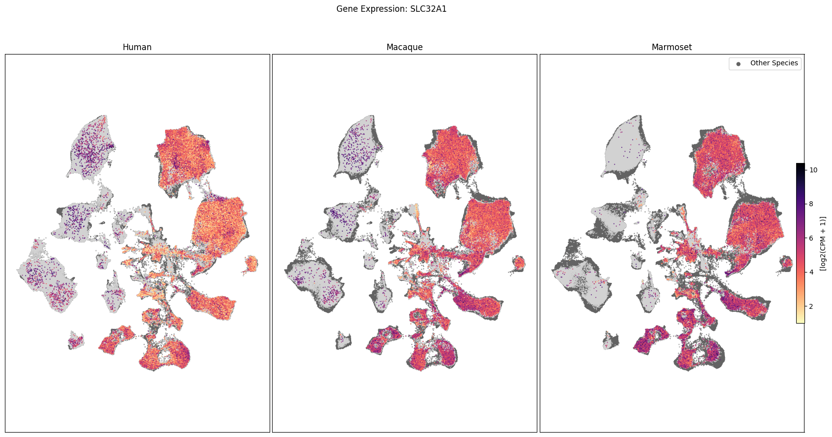
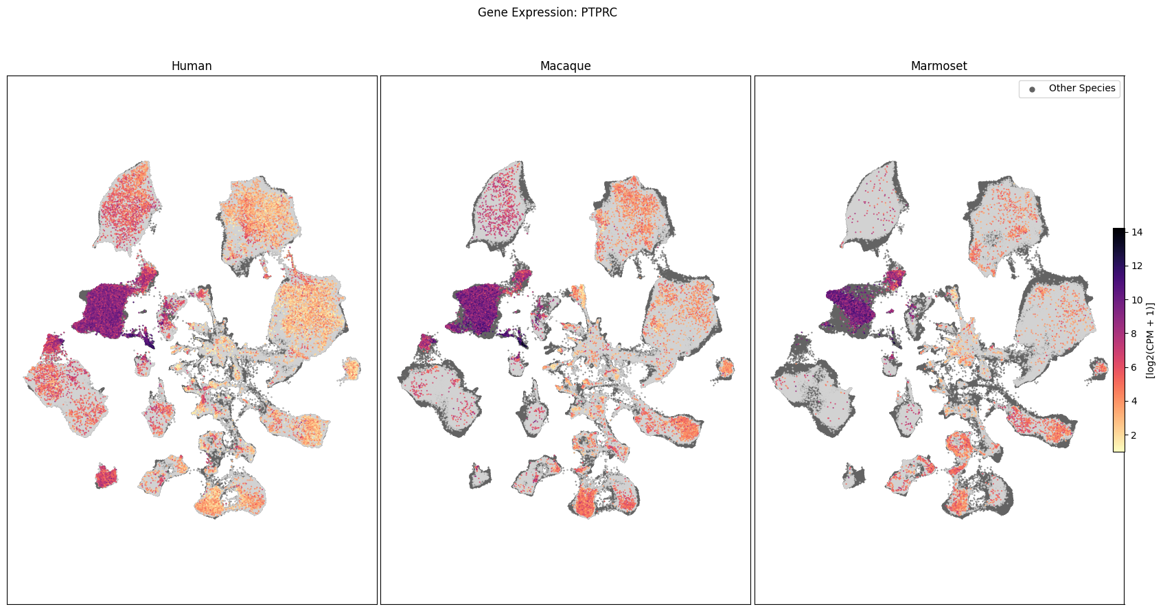
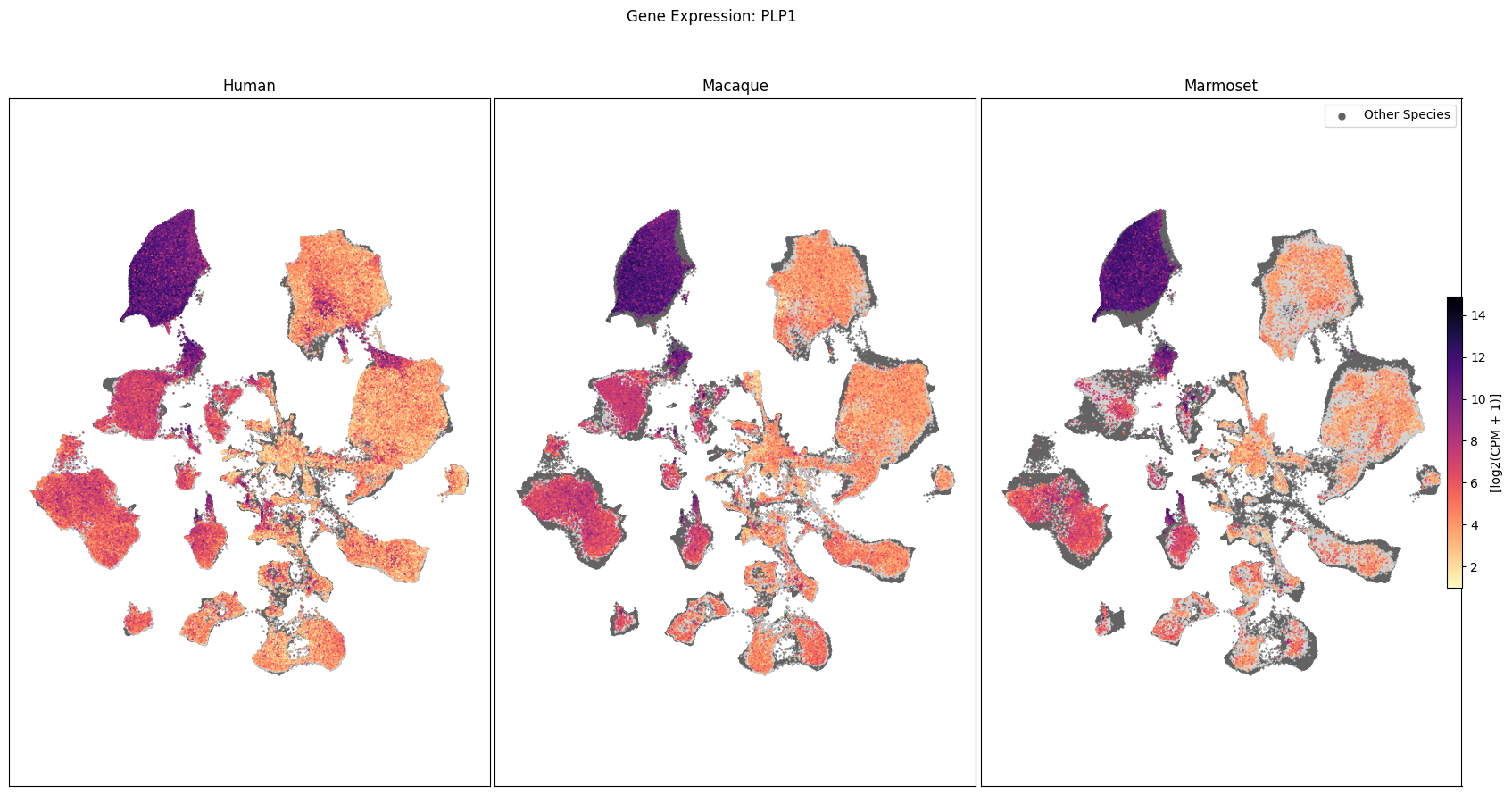
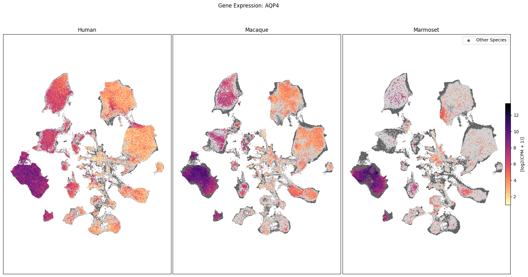
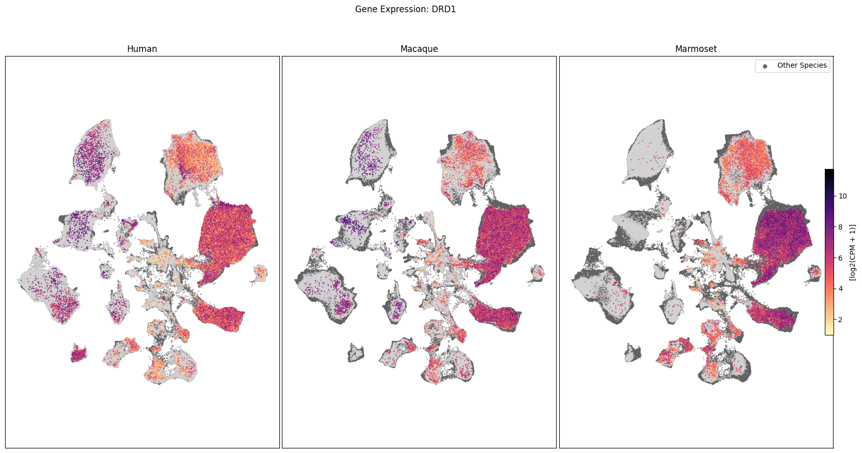
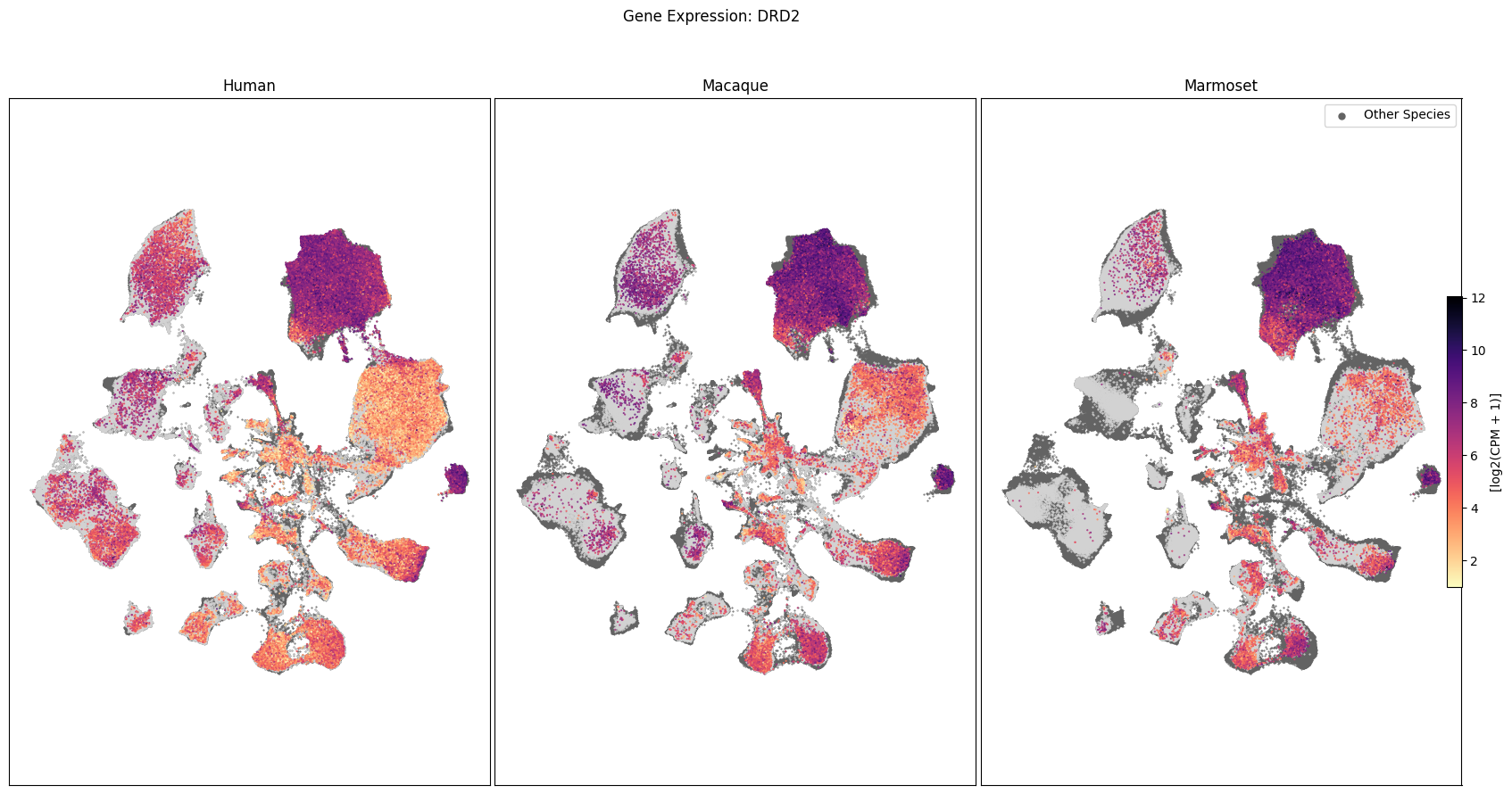
In this section, we show a use case with the example genes SLC17A6, SLC32A1, PTPRC, PLP1, AQP4, DRD1, and DRD2. These genes were selected because they are marker genes for glutamatergic (SLC17A6) and GABAergic (SLC32A1) neurons, immune cells (PTPRC), oligodendrocytes (PLP1), astrocytes (AQP4), and D1/D2 medium spiny neurons (DRD1, DRD2). “Marker genes” have much higher expression in the specified cell type or anatomic structure when compared to all other cells, and in many cases are functionally relevant for those cell types.

We define a helper functions aggregate_by_metadata to compute the average expression for a given category and later plot_umap to plot cells in a UMAP colorized by metadata or expression values similar to what was used in part 1.

The helper function below creates a heatmap showing the relation between various parameters in the combined cell metadata and the genes we loaded.

def plot_species_heatmap(
    df,
    gnames,
    value,
    species_list=None,
    sort=False,
    fig_width=8,
    fig_height=4,
    vmax=None,
    cmap=plt.cm.magma_r
):
    if species_list is None:
        species_list = df['species_common_name'].unique()

    fig, ax = plt.subplots(1, len(species_list))
    fig.set_size_inches(fig_width, fig_height)

    all_unique_values = df[value].unique()
    try:
        order = df[f'{value}_order'].unique()
        all_unique_values = all_unique_values[np.argsort(order)]
    except KeyError:
        order = None

    for idx, species in enumerate(species_list):
        
        filtered = df[df['species_common_name'] == species]
        
        grouped = filtered.groupby(value)[gnames].mean()
        if sort:
            grouped = grouped.sort_values(by=gnames[0], ascending=False)

        missing_values = []
        indices = []
        for unique_value in all_unique_values:
            if unique_value not in grouped.index:        
                indices.append(unique_value)
                missing_values.append({key: np.nan for key in gnames})

        if missing_values:
            grouped = pd.concat([grouped, pd.DataFrame(data=missing_values, index=indices)])
        grouped = grouped.loc[all_unique_values]

        arr = grouped.to_numpy().astype('float')

        ax[idx].imshow(arr, cmap=cmap, aspect='auto', vmin=0, vmax=vmax)
        xlabs = grouped.columns.values
        ylabs = grouped.index.values

        if idx == 0:
            ax[idx].set_yticks(range(len(ylabs)))
            ax[idx].set_yticklabels(ylabs)
        else:
            ax[idx].set_yticks([])
            ax[idx].set_yticklabels([])
        ax[idx].set_xticks(range(len(xlabs)))
        ax[idx].set_xticklabels(xlabs)
        ax[idx].set_title(species)

    plt.subplots_adjust(wspace=0.00, hspace=0.00)
    
    return fig, ax

Expression of selected genes in the Basal Ganglia

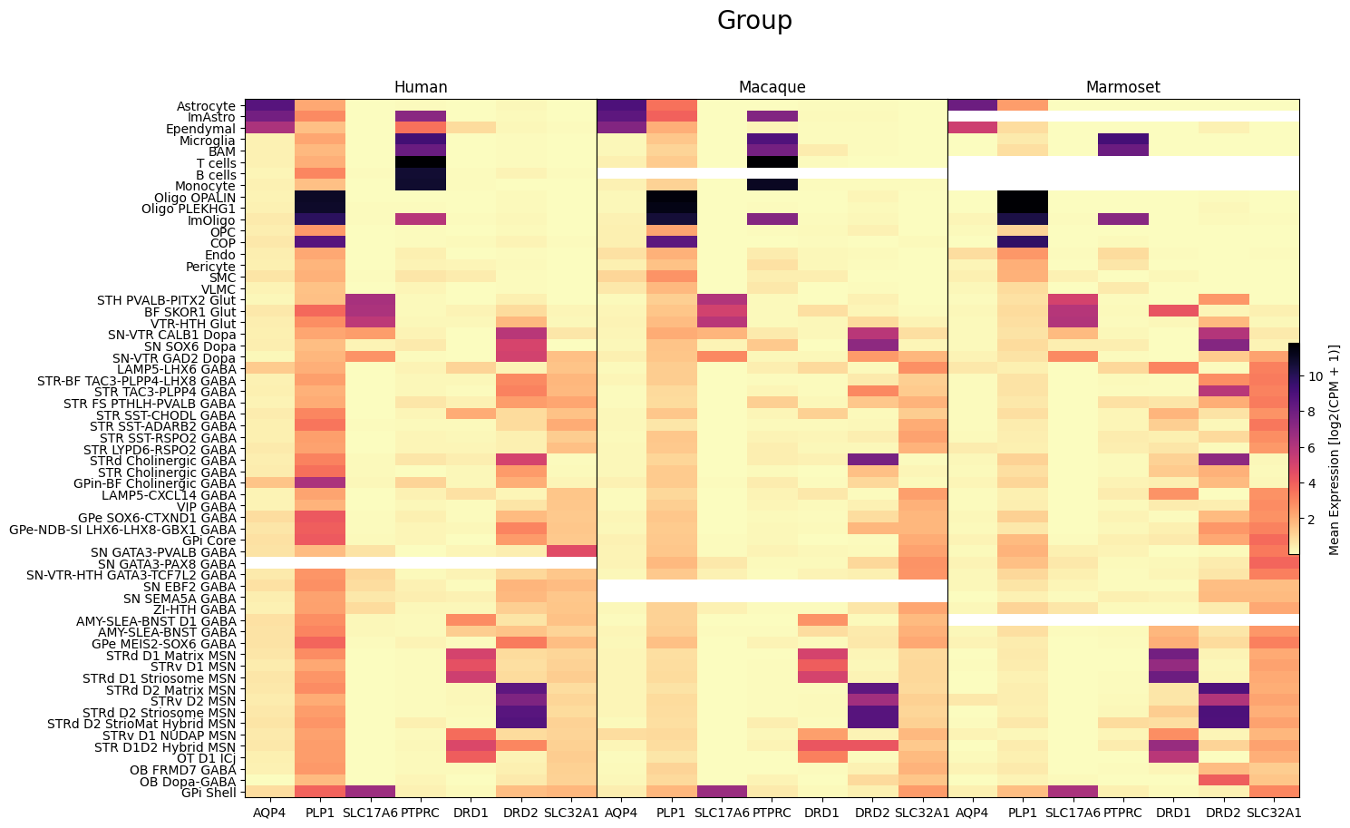
Below we use our heatmap function to plot the gene expression as a function of a feature in our data. For the first two plots, we show the expression for all species against the Neighborhood and Group levels of the taxonomy. We observe that the expression across the species are similar as we would expect if these cell types are conserved across species. Note that a band of white denotes a Group (or other feature) that is not present in for the given species.

fig, ax = plot_species_heatmap(
    df=cell_extended_with_genes,
    gnames=aligned_gene_data.columns,
    value='Neighborhood',
    species_list=['Human', 'Macaque', 'Marmoset'],
    fig_width=15,
    fig_height=5
)
fig.suptitle('Neighborhood')
plt.show()

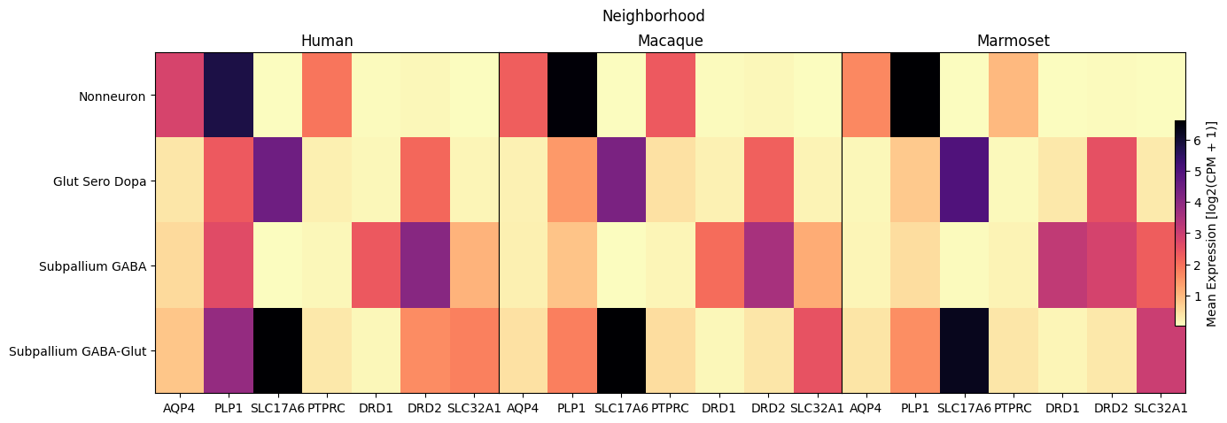
fig, ax = plot_species_heatmap(
    df=cell_extended_with_genes,
    gnames=aligned_gene_data.columns,
    value='Group',
    species_list=['Human', 'Macaque', 'Marmoset'],
    fig_width=15,
    fig_height=10
)
fig.suptitle('Group', size=20)
plt.show()

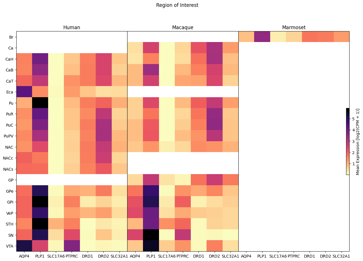
Now we perform the same heatmap comparison against the region of interest in the brain the cell was extracted from. Note that currently the Marmoset has no fine grained identification of brain region.

fig, ax = plot_species_heatmap(
    df=cell_extended_with_genes,
    gnames=aligned_gene_data.columns,
    species_list=['Human', 'Macaque', 'Marmoset'],
    value='region_of_interest_label',
    fig_width=15,
    fig_height=10
)
fig.suptitle('Region of Interest')
plt.show()

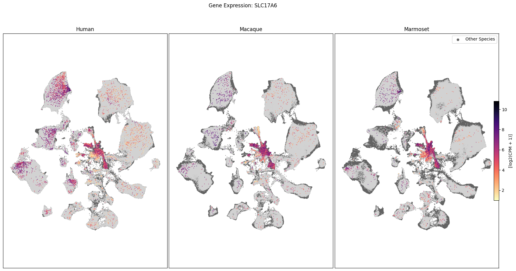
Expression in the UMAP

We can also visualize the relationship between these genes and their location in the UMAP. We’ll plot the two species side by side with the lightgrey cells in each plot representing those from the other species that do not overlap with the plotted one. Overall the expressions between species agree across the UMAP.

def plot_umap(df, feature, species_list, cmap=None, fig_width=21, fig_height=10) :
    
    fig, ax = plt.subplots(1, len(species_list))
    fig.set_size_inches(fig_width, fig_height)

    all_xx = df['x']
    all_yy = df['y']
    
    for idx, species in enumerate(species_list):
        
        filtered = df[df['species_common_name'] == species]
        xx = filtered['x']
        yy = filtered['y']
        vv = filtered[feature]
        ax[idx].scatter(all_xx, all_yy, s=1.0, color='#D3D3D3', marker='.')
        
        if cmap is not None :
            ax[idx].scatter(xx, yy, s=1.0, c=vv, marker='.', cmap=cmap)
        else :
            ax[idx].scatter(xx, yy, s=1.0, color=vv, marker=".")
            
        ax[idx].axis('equal')
        ax[idx].set_xticks([])
        ax[idx].set_yticks([])
        
        ax[idx].set_title(f"{species}")
        
    plt.subplots_adjust(wspace=0.01, hspace=0.01)
    return fig, ax

for gene_name in gene_names:
    fig, ax = plot_umap(
        cell_extended_with_genes,
        feature=gene_name,
        species_list=['Human', 'Macaque', 'Marmoset'],
        cmap=plt.cm.magma_r
    )
    fig.suptitle(f'Gene Expression: {gene_name}')
    plt.show()