10x RNA-seq clustering analysis and annotation (CCN20230722)

The Mouse Whole Brain Atlas is a high-resolution transcriptomic and spatial cell-type atlas across the entire mouse brain, integrating several whole-brain single-cell RNA-sequencing (scRNA-seq) datasets. The datasets contain a total of ~4 million cells passing rigorous quality-control (QC) criteria. The integrated transcriptomic taxonomy contains 5,322 clusters that are organized in a hierarchical manner with nested groupings of 34 classes, 338 subclasses, 1,201 supertypes and 5,322 types/clusters. The scRNA-seq data reveal transcriptome-wide gene expression and co-expression patterns for each cell type. The anatomical location of each cell type has been annotated using a comprehensive brain-wide MERFISH dataset with a total of ~4 million segmented and QC-passed cells, probed with a 500-gene panel and registered to the Allen Mouse Brain Common Coordinate Framework (CCF v3). The MERFISH data not only provide accurate spatial annotation of cell types at subclass, supertype and cluster levels, but also reveal fine-resolution spatial distinctions or gradients for cell types. The combination of scRNA-seq and MERFISH data reveals a high degree of correspondence between transcriptomic identity and spatial specificity for each cell type, as well as unique features of cell type organization in different brain regions.

The purpose of this notebook is to provide an overview of how cluster and cluster annotation information is represented through example use cases.

You need to be connected to the internet to run this notebook and that you have already downloaded the data via the getting started notebook.

A detailed cell type annotation table is also provided along with data downloads detailing information about the hierarchical membership, anatomical annotation, neurotransmitter type, cell type marker genes, transcription factor and neuropeptide markers, and other metadata types for each cluster.

import os
import pandas as pd
import numpy as np
import matplotlib.pyplot as plt
import pathlib

from abc_atlas_access.abc_atlas_cache.abc_project_cache import AbcProjectCache

We will interact with the data using the AbcProjectCache. This cache object tracks which data has been downloaded and serves the path to the requsted data on disk. For metadata, the cache can also directly serve a up a Pandas Dataframe. See the getting_started notebook for more details on using the cache including installing it if it has not already been.

Change the download_base variable to where you have downloaded the data in your system.

download_base = pathlib.Path('../../abc_download_root')
abc_cache = AbcProjectCache.from_s3_cache(download_base)
abc_cache.current_manifest

'releases/20240330/manifest.json'

Data Overview

Clusters

Each of the final set of 5196 cluster is associated with an alias and label. Each row of the dataframe represnts a cluster. Each cluster has a label (human readable string that is unique in the database), cluster alias (in this case a simple integer) and the number of cells that has been grouped into the cluster.

cluster = abc_cache.get_metadata_dataframe(directory='WMB-taxonomy', file_name='cluster')
print(len(cluster))
cluster.head(5)

5322

	cluster_alias	number_of_cells	label
0	1	727	CS20230722_0001
1	10	740	CS20230722_0010
2	100	1053	CS20230722_0100
3	1000	59	CS20230722_1000
4	1001	96	CS20230722_1001

Cluster annotation term sets

Each level of classification is represented as a cluster annotation term set. Each term set consists of a set of ordered terms. Each term set has a label (human readable string that is unique in the database), a name, description and order among the term sets. Note that these are terms specific to the WMB dataset. The WHB dataset contains supercluster, cluster, subcluster, and neurotransmitter. See the WHB cluster annotation tutorial for more information.

term_set = abc_cache.get_metadata_dataframe(directory='WMB-taxonomy', file_name='cluster_annotation_term_set')
term_set

	label	name	description	order
0	CCN20230722_NEUR	neurotransmitter	Clusters are assigned based on the average exp...	0
1	CCN20230722_CLAS	class	The top level of cell type definition in the m...	1
2	CCN20230722_SUBC	subclass	The coarse level of cell type definition in th...	2
3	CCN20230722_SUPT	supertype	The second finest level of cell type definitio...	3
4	CCN20230722_CLUS	cluster	The finest level of cell type definition in th...	4

We can use the pandas iterrows function to print out the description for each term set.

# print out description for each term_set
for tsindex, tsrow in term_set.iterrows() :
    print("%s:\n" % tsrow['name'])
    print("%s\n" % tsrow['description'])

neurotransmitter:

Clusters are assigned based on the average expression of both neurotransmitter transporter genes and key neurotransmitter synthesizing enzyme genes.

class:

The top level of cell type definition in the mouse whole brain taxonomy. It is primarily determined by broad brain region and neurotransmitter type. All cells within a subclass belong to the same class. Class provides a broader categorization of cell types.

subclass:

The coarse level of cell type definition in the mouse whole brain taxonomy. All cells within a supertype belong to the same subclass. Subclass groups together related supertypes.

supertype:

The second finest level of cell type definition in the mouse whole brain taxonomy. All cells within a cluster belong to the same supertype. Supertype groups together similar clusters.

cluster:

The finest level of cell type definition in the mouse whole brain taxonomy. Cells within a cluster share similar characteristics and belong to the same supertype.

Cluster annotation terms

A cluster annotation term represents a group within a single level of classification. Each term object has a label (human readable string that is unique in the database), a name, which cluster annotation term set it belongs to and a parent or superclass if the term forms a heirarchy, an order within a term set and a color for visualization purposes.

term = abc_cache.get_metadata_dataframe(directory='WMB-taxonomy', file_name='cluster_annotation_term', keep_default_na=False)
term.head(5)

	label	name	cluster_annotation_term_set_label	parent_term_label	parent_term_set_label	term_set_order	term_order	cluster_annotation_term_set_name	color_hex_triplet
0	CS20230722_NEUR_Glut	Glut	CCN20230722_NEUR			0	0	neurotransmitter	#2B93DF
1	CS20230722_NEUR_NA	NA	CCN20230722_NEUR			0	1	neurotransmitter	#666666
2	CS20230722_NEUR_GABA	GABA	CCN20230722_NEUR			0	2	neurotransmitter	#FF3358
3	CS20230722_NEUR_Dopa	Dopa	CCN20230722_NEUR			0	3	neurotransmitter	#fcf04b
4	CS20230722_NEUR_Glut-GABA	Glut-GABA	CCN20230722_NEUR			0	4	neurotransmitter	#0a9964

We can use the groupby and count functions in pandas to tally the number of terms in each term set (classification level).

term[['label','cluster_annotation_term_set_name']].groupby('cluster_annotation_term_set_name').count()

	label
cluster_annotation_term_set_name
class	34
cluster	5322
neurotransmitter	10
subclass	338
supertype	1201

It is important to note that term names are only unique within a term set and not unique across term sets. In particular, the name “0001 CLA-EPd-CTX Car3 Glut_1” is used both as supertype and cluster term. These are distinct entities as supertype “0001 CLA-EPd-CTX Car3 Glut_1” has three other distinct cluster members. As such when doing aggregation operations, it is important to the use the term label instead of name. For the name “0001 CLA-EPd-CTX Car3 Glut_1”, the associated label terms are ” CS20230722_SUPT_0001” and “CS20230722_CLUS_000” in the supertype and class level respectively.

# Use the groupby function to find the usage count for each term name
term_name_count = term.groupby(['name'])[['cluster_annotation_term_set_name']].count()
term_name_count.columns = ['usage_count']
pred = term_name_count['usage_count'] > 1
term_name_count = term_name_count[pred]
term_name_count

	usage_count
name
0001 CLA-EPd-CTX Car3 Glut_1	2

# Filter the dataframe to terms where there was a name reuse
pred = [x in term_name_count.index for x in term['name']]
name_clash_term = term[pred][['label','name','cluster_annotation_term_set_name']]
name_clash_term

	label	name	cluster_annotation_term_set_name
382	CS20230722_SUPT_0001	0001 CLA-EPd-CTX Car3 Glut_1	supertype
1583	CS20230722_CLUS_0001	0001 CLA-EPd-CTX Car3 Glut_1	cluster

# List all clusters which have supertype "0001 CLA-EPd-CTX Car3 Glut_1" as parent
pred = (term['parent_term_label'] == 'CS20230722_SUPT_0001')
term[pred]

	label	name	cluster_annotation_term_set_label	parent_term_label	parent_term_set_label	term_set_order	term_order	cluster_annotation_term_set_name	color_hex_triplet
1583	CS20230722_CLUS_0001	0001 CLA-EPd-CTX Car3 Glut_1	CCN20230722_CLUS	CS20230722_SUPT_0001	CCN20230722_SUPT	4	0	cluster	#00664E
1584	CS20230722_CLUS_0002	0002 CLA-EPd-CTX Car3 Glut_1	CCN20230722_CLUS	CS20230722_SUPT_0001	CCN20230722_SUPT	4	1	cluster	#5C79CC
1585	CS20230722_CLUS_0003	0003 CLA-EPd-CTX Car3 Glut_1	CCN20230722_CLUS	CS20230722_SUPT_0001	CCN20230722_SUPT	4	2	cluster	#86FF4D
1586	CS20230722_CLUS_0004	0004 CLA-EPd-CTX Car3 Glut_1	CCN20230722_CLUS	CS20230722_SUPT_0001	CCN20230722_SUPT	4	3	cluster	#CC563D

Cluster to cluster annotation membership

The association between a cluster and cluster annotation term is represented as a cluster to cluster annotation membership within the context of one cluster annotation term set. It is expected that a cluster in only associated with one term within a specific term set.

membership = abc_cache.get_metadata_dataframe(directory='WMB-taxonomy', file_name='cluster_to_cluster_annotation_membership')
membership.head(5)

	cluster_annotation_term_label	cluster_annotation_term_set_label	cluster_alias	cluster_annotation_term_name	cluster_annotation_term_set_name	number_of_cells	color_hex_triplet
0	CS20230722_CLUS_0001	CCN20230722_CLUS	128	0001 CLA-EPd-CTX Car3 Glut_1	cluster	4262	#00664E
1	CS20230722_CLUS_0002	CCN20230722_CLUS	129	0002 CLA-EPd-CTX Car3 Glut_1	cluster	3222	#5C79CC
2	CS20230722_CLUS_0003	CCN20230722_CLUS	130	0003 CLA-EPd-CTX Car3 Glut_1	cluster	12216	#86FF4D
3	CS20230722_CLUS_0004	CCN20230722_CLUS	143	0004 CLA-EPd-CTX Car3 Glut_1	cluster	9334	#CC563D
4	CS20230722_CLUS_0005	CCN20230722_CLUS	131	0005 CLA-EPd-CTX Car3 Glut_2	cluster	1056	#E7FF26

Example use cases

Aggregating cluster and cells counts per term

We can obtain cluster and cell counts per cluster annotation term using the pandas groupby function.

# Count the number of clusters associated with each cluster annotation term
term_cluster_count = membership.groupby(['cluster_annotation_term_label'])[['cluster_alias']].count()
term_cluster_count.columns = ['number_of_clusters']
term_cluster_count.head(5)

	number_of_clusters
cluster_annotation_term_label
CS20230722_CLAS_01	402
CS20230722_CLAS_02	83
CS20230722_CLAS_03	16
CS20230722_CLAS_04	16
CS20230722_CLAS_05	105

# Sum up the number of cells associated with each cluster annotation term
term_cell_count = membership.groupby(['cluster_annotation_term_label'])[['number_of_cells']].sum()
term_cell_count.columns = ['number_of_cells']
term_cell_count.head(5)

	number_of_cells
cluster_annotation_term_label
CS20230722_CLAS_01	1095484
CS20230722_CLAS_02	310198
CS20230722_CLAS_03	4767
CS20230722_CLAS_04	84352
CS20230722_CLAS_05	107502

# Join counts with the term dataframe
term_by_label = term.set_index('label')
term_with_counts = term_by_label.join(term_cluster_count)
term_with_counts = term_with_counts.join(term_cell_count)
term_with_counts[['name', 'cluster_annotation_term_set_name', 'number_of_clusters', 'number_of_cells']].head(5)

	name	cluster_annotation_term_set_name	number_of_clusters	number_of_cells
label
CS20230722_NEUR_Glut	Glut	neurotransmitter	2561	2054137
CS20230722_NEUR_NA	NA	neurotransmitter	127	1089152
CS20230722_NEUR_GABA	GABA	neurotransmitter	1991	834601
CS20230722_NEUR_Dopa	Dopa	neurotransmitter	67	9396
CS20230722_NEUR_Glut-GABA	Glut-GABA	neurotransmitter	62	8989

The term_with_counts datafarme is available in the cache as cluster_annotation_term_with_counts.

Let’s visualize cluster and cells counts for of the classification levels using bar plots.

def bar_plot_by_level_and_type(df, level, fig_width = 8.5, fig_height = 4):
    
    fig, ax = plt.subplots(1, 2)
    fig.set_size_inches(fig_width, fig_height)
    
    for idx, ctype in enumerate(['clusters', 'cells']):

        pred = (df['cluster_annotation_term_set_name'] == level )
        names = df[pred]['name']
        counts = df[pred]['number_of_%s' % ctype]
        colors = df[pred]['color_hex_triplet']
        
        ax[idx].barh(names, counts, color=colors)
        ax[idx].set_title('Number of %s by %s' % (ctype,level)),
        ax[idx].set_xscale('log')
        
        if idx > 0 :
            ax[idx].set_yticklabels([])

    plt.show()

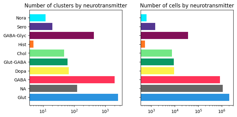
Neurotransmitter cluster and cell counts

The majority of clusters and cells are of glutamatergic, GABAergic or GABA-glycinergic neurotransmitter types.

df = term_with_counts
level = 'neurotransmitter'
pred = (df['cluster_annotation_term_set_name'] == level )

bar_plot_by_level_and_type(term_with_counts, 'neurotransmitter')

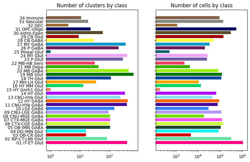
Class level cluster and cell counts

Class “18 MB Glut” contains the largest number of clusters (>600), while class “01 IT-ET Glut” contains the largest number of cells (>1.0 million).

bar_plot_by_level_and_type(term_with_counts, 'class', 8.5, 6)

Visualizing cluster and term distributions

We can explore the relationship and distribution of clusters between term sets by creating a pivot table using pandas groupby fuunction. Each row of the resulting dataframe represents a cluster, each column represents a term set and the value in the table is the name of the term that has been associated with the cluster for that specific term set.

pivot = membership.groupby(['cluster_alias', 'cluster_annotation_term_set_name'])['cluster_annotation_term_name'].first().unstack()
pivot = pivot[term_set['name']] # order columns
pivot

cluster_annotation_term_set_name	neurotransmitter	class	subclass	supertype	cluster
cluster_alias
1	Glut	01 IT-ET Glut	018 L2 IT PPP-APr Glut	0082 L2 IT PPP-APr Glut_3	0326 L2 IT PPP-APr Glut_3
2	Glut	01 IT-ET Glut	018 L2 IT PPP-APr Glut	0082 L2 IT PPP-APr Glut_3	0327 L2 IT PPP-APr Glut_3
3	Glut	01 IT-ET Glut	018 L2 IT PPP-APr Glut	0081 L2 IT PPP-APr Glut_2	0322 L2 IT PPP-APr Glut_2
4	Glut	01 IT-ET Glut	018 L2 IT PPP-APr Glut	0081 L2 IT PPP-APr Glut_2	0323 L2 IT PPP-APr Glut_2
5	Glut	01 IT-ET Glut	018 L2 IT PPP-APr Glut	0081 L2 IT PPP-APr Glut_2	0325 L2 IT PPP-APr Glut_2
...	...	...	...	...	...
34368	GABA-Glyc	27 MY GABA	288 MDRN Hoxb5 Ebf2 Gly-Gaba	1102 MDRN Hoxb5 Ebf2 Gly-Gaba_1	4955 MDRN Hoxb5 Ebf2 Gly-Gaba_1
34372	GABA-Glyc	27 MY GABA	285 MY Lhx1 Gly-Gaba	1091 MY Lhx1 Gly-Gaba_3	4901 MY Lhx1 Gly-Gaba_3
34374	GABA-Glyc	27 MY GABA	285 MY Lhx1 Gly-Gaba	1091 MY Lhx1 Gly-Gaba_3	4902 MY Lhx1 Gly-Gaba_3
34376	GABA-Glyc	27 MY GABA	285 MY Lhx1 Gly-Gaba	1091 MY Lhx1 Gly-Gaba_3	4903 MY Lhx1 Gly-Gaba_3
34380	GABA-Glyc	27 MY GABA	285 MY Lhx1 Gly-Gaba	1095 MY Lhx1 Gly-Gaba_7	4924 MY Lhx1 Gly-Gaba_7

5322 rows × 5 columns

We can also obtain a cluster annotation color pivot table in the same way.

color = membership.groupby(['cluster_alias','cluster_annotation_term_set_name'])['color_hex_triplet'].first().unstack().fillna('#f9f9f9')
color = color[term_set['name']] # order columns
color.columns = ['%s_color' % x for x in color.columns]
color

	neurotransmitter_color	class_color	subclass_color	supertype_color	cluster_color
cluster_alias
1	#2B93DF	#FA0087	#0F6632	#266DFF	#64661F
2	#2B93DF	#FA0087	#0F6632	#266DFF	#CCA73D
3	#2B93DF	#FA0087	#0F6632	#002BCC	#99000D
4	#2B93DF	#FA0087	#0F6632	#002BCC	#5C8899
5	#2B93DF	#FA0087	#0F6632	#002BCC	#473D66
...	...	...	...	...	...
34368	#820e57	#0096C7	#660038	#5CCCA4	#500099
34372	#820e57	#0096C7	#f20985	#976df9	#0F6627
34374	#820e57	#0096C7	#f20985	#976df9	#2E4799
34376	#820e57	#0096C7	#f20985	#976df9	#15FF00
34380	#820e57	#0096C7	#f20985	#FF2B26	#459988

5322 rows × 5 columns

The pivot and color dataframes created above are stored in the cache as cluster_to_cluster_annotation_membership_pivoted and cluster_to_cluster_annotation_membership_color respectively.

For a given pair of term sets A and B, define a function distribution that creates a cluster count table where the rows are terms in term set A, columns are terms in term set B and the table values being the number of clusters that is shared between the terms.

def distribution(A, B) :
    
    AxB = pivot.groupby([A,B])[['cluster']].count()
    AxB.columns = ['number_of_clusters']
    AxB = AxB.unstack().fillna(0)

    B_names = [x[1] for x in list(AxB.columns)]
    pred = (term['cluster_annotation_term_set_name'] == B)
    term_by_name = term[pred].set_index('name')
    B_colors = term_by_name.loc[B_names, 'color_hex_triplet']
    
    return AxB, B_names, B_colors

Function stacked_bar_distribution takes the results of distribution as input to create distribution stacked bar plot.

def stacked_bar_distribution(AxB, B_names, B_colors, fig_width = 6, fig_height = 6):

    fig, ax = plt.subplots()
    fig.set_size_inches(fig_width, fig_height)

    bottom = np.zeros(len(AxB))

    for i, col in enumerate(AxB.columns):
        ax.barh(AxB.index, AxB[col], left=bottom, label=col[1], color=B_colors[i])
        bottom += np.array(AxB[col])

    ax.set_title('Distribution of %s in each %s' % (AxB.columns.names[1], AxB.index.name))
    ax.legend(loc='center left', bbox_to_anchor=(1, 0.5))

    plt.show()
    
    return fig, ax

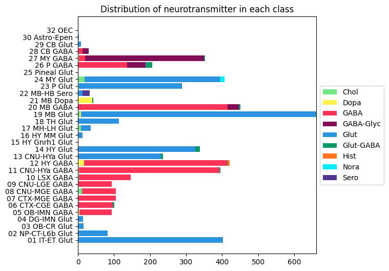
Distribution of neurotransmitter clusters in each class

At the next level of classification, around 50% of the classes are have a single neurotransmitter identity and remaining 50% are of mixed types.

AxB, B_names, B_colors = distribution('class', 'neurotransmitter')
fig, ax = stacked_bar_distribution(AxB, B_names, B_colors, 6, 6)

/var/folders/kc/7glrmt5n67x16yj_tg86t49c0000gp/T/ipykernel_77026/1772253940.py:9: FutureWarning: Series.__getitem__ treating keys as positions is deprecated. In a future version, integer keys will always be treated as labels (consistent with DataFrame behavior). To access a value by position, use `ser.iloc[pos]`
  ax.barh(AxB.index, AxB[col], left=bottom, label=col[1], color=B_colors[i])

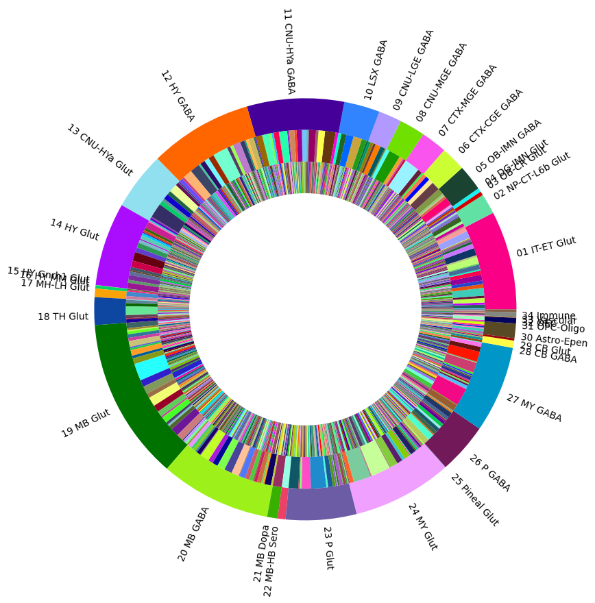
Visualizing the mouse whole brain taxonomy

Term sets: class, subclass, supertype and cluster forms a four level mouse whole brain taxonomy. We can visualized the taxonomy as a sunburst diagram that shows the single inheritance hierarchy through a series of rings, that are sliced for each annotation term. Each ring corresponds to a level in the hierarchy. We have ordered the rings so that the class level is the outer most ring so that we can add in labels. Rings are sliced up and divided based on their hierarchical relationship to the parent slice. The angle of each slice is proportional to the number of clusters belonging to the term.

levels = ['class', 'subclass', 'supertype']
df = {}

for lvl in levels:
    pred = term_with_counts['cluster_annotation_term_set_name'] == lvl
    df[lvl] = term_with_counts[pred]
    df[lvl] = df[lvl].sort_values(['parent_term_label', 'label'])

fig, ax = plt.subplots()
fig.set_size_inches(10, 10)
size = 0.15

for i, lvl in enumerate(levels):
    
    if lvl == 'class':
        ax.pie(df[lvl]['number_of_clusters'],
               colors=df[lvl]['color_hex_triplet'],
               labels = df[lvl]['name'],
               rotatelabels=True,
               labeldistance=1.025,
               radius=1,
               wedgeprops=dict(width=size, edgecolor=None),
               startangle=0)
    else :
        ax.pie(df[lvl]['number_of_clusters'],
               colors=df[lvl]['color_hex_triplet'],
               radius=1-i*size,
               wedgeprops=dict(width=size, edgecolor=None),
               startangle=0)

plt.show()