Whole Human Brain (WHB) 10x RNA-seq gene expression data (part 1)#
The purpose of this set of notebooks is to provide an overview of the data, the file organization, and how to combine data and metadata through example use cases.
You need to be connected to the internet to run this notebook or connected to a cache that has the WHB data downloaded already.
The notebook presented here shows quick visualizations from precomputed metadata in the atlas. For examples on accesing the expression matricies, specifically selecting genes from expression matricies, see the general_acessing_10x_snRNASeq_tutorial.ipynb tutorial/example.
For full details of the data, see Siletti et al. 2023.
import pandas as pd
from pathlib import Path
import numpy as np
import anndata
import matplotlib.pyplot as plt

from abc_atlas_access.abc_atlas_cache.abc_project_cache import AbcProjectCache
We will interact with the data using the AbcProjectCache. This cache object tracks which data has been downloaded and serves the path to the requsted data on disk. For metadata, the cache can also directly serve a up a Pandas Dataframe. See the getting_started notebook for more details on using the cache including installing it if it has not already been.
Change the download_base variable to where you have downloaded the data in your system.
download_base = Path('../../data/abc_atlas')
abc_cache = AbcProjectCache.from_cache_dir(download_base)

abc_cache.current_manifest
'releases/20250531/manifest.json'
Data overview#
Cell metadata#
Essential cell metadata is stored as a dataframe. Each row represents one cell indexed by a cell label. The cell label is the concatenation of barcode and name of the sample. In this context, the sample is the barcoded cell sample that represents a single load into one port of the 10x Chromium. Note that cell barcodes are only unique within a single barcoded cell sample and that the same barcode can be reused. The barcoded cell sample label or name is unique in the database.
Each cell is associated with a library label, library method, donor label, donor sex, dissection region_of_interest_label, the corresponding coarse anatomical division label and the matrix_prefix identifying which data package this cell is part of.
Further, each cell is associated with a cluster alias representing which cluster this cell is a member of and (x, y) coordinates of the cells UMAP in Figure 1B of Siletti et al. The neurons and non-neurons in the cells table have overlapping (x, y) coordinates and should be plotted seperately.
Below, we load the first of the metadata used in this tutorial. This pattern of loading metadata is repeated throughout the tutorials.
abc_cache.list_metadata_files('WHB-10Xv3')
['anatomical_division_structure_map',
 'cell_metadata',
 'donor',
 'example_genes_all_cells_expression',
 'gene',
 'region_of_interest_structure_map']
abc_cache.list_metadata_files('WHB-taxonomy')
['cluster',
 'cluster_annotation_term',
 'cluster_annotation_term_set',
 'cluster_to_cluster_annotation_membership']
cell = abc_cache.get_metadata_dataframe(
    directory='WHB-10Xv3',
    file_name='cell_metadata',
    dtype={'cell_label': str}
)
cell.set_index('cell_label', inplace=True)
print("Number of cells = ", len(cell))
cell.head(5)
cell.columns
Number of cells = 3369219
Index(['cell_barcode', 'barcoded_cell_sample_label', 'library_label',
       'feature_matrix_label', 'entity', 'brain_section_label',
       'library_method', 'donor_label', 'donor_sex', 'dataset_label', 'x', 'y',
       'cluster_alias', 'region_of_interest_label',
       'anatomical_division_label', 'abc_sample_id'],
      dtype='object')
We can use pandas groupby function to see how many unique items are associated for each field and list them out if the number of items is small.
def print_column_info(df):

    for c in df.columns:
        grouped = df[[c]].groupby(c).count()
        members = ''
        if len(grouped) < 30:
            members = str(list(grouped.index))
        print("Number of unique %s = %d %s" % (c, len(grouped), members))
print_column_info(cell)
Number of unique cell_barcode = 2205155
Number of unique barcoded_cell_sample_label = 606
Number of unique library_label = 606
Number of unique feature_matrix_label = 2 ['WHB-10Xv3-Neurons', 'WHB-10Xv3-Nonneurons']
Number of unique entity = 1 ['nuclei']
Number of unique brain_section_label = 57
Number of unique library_method = 1 ['10Xv3']
Number of unique donor_label = 4 ['H18.30.001', 'H18.30.002', 'H19.30.001', 'H19.30.002']
Number of unique donor_sex = 2 ['F', 'M']
Number of unique dataset_label = 1 ['WHB-10Xv3']
Number of unique x = 3369219
Number of unique y = 3369219
Number of unique cluster_alias = 3313
Number of unique region_of_interest_label = 109
Number of unique anatomical_division_label = 14 ['Amygdaloid complex', 'Basal forebrain', 'Basal nuclei', 'Cerebellum', 'Cerebral cortex', 'Claustrum', 'Extended amygdala', 'Hippocampus', 'Hypothalamus', 'Midbrain', 'Myelencephalon', 'Pons', 'Spinal cord', 'Thalamus']
Number of unique abc_sample_id = 3369219
cell.groupby('dataset_label')[['x']].count()
| x | |
|---|---|
| dataset_label | |
| WHB-10Xv3 | 3369219 |
We can also create a pivot table to associate each cell with terms at each cell type classification level. To do this we need to load multiple other metadata tables and join them into the main cells table. See the cluster annotation tutorial for more details.
membership = abc_cache.get_metadata_dataframe(
    directory='WHB-taxonomy',
    file_name='cluster_to_cluster_annotation_membership'
)
membership_groupby = membership.groupby(['cluster_alias', 'cluster_annotation_term_set_name'])
membership.head(5)
| cluster_annotation_term_label | cluster_annotation_term_set_label | cluster_alias | cluster_annotation_term_name | cluster_annotation_term_set_name | number_of_cells | color_hex_triplet | |
|---|---|---|---|---|---|---|---|
| 0 | CS202210140_494 | CCN202210140_SUBC | 0 | URL_297_0 | subcluster | 34 | #7E807A |
| 1 | CS202210140_495 | CCN202210140_SUBC | 1 | URL_308_1 | subcluster | 220 | #C54945 |
| 2 | CS202210140_496 | CCN202210140_SUBC | 2 | URL_308_2 | subcluster | 187 | #5232B7 |
| 3 | CS202210140_497 | CCN202210140_SUBC | 3 | URL_308_3 | subcluster | 246 | #31BEBA |
| 4 | CS202210140_498 | CCN202210140_SUBC | 4 | URL_308_4 | subcluster | 188 | #C8A9BC |
term_sets = abc_cache.get_metadata_dataframe(directory='WHB-taxonomy', file_name='cluster_annotation_term_set').set_index('label')
cluster_details = membership_groupby['cluster_annotation_term_name'].first().unstack()
cluster_details = cluster_details[term_sets['name']] # order columns
cluster_details.fillna('Other', inplace=True)
cluster_details.sort_values(['supercluster', 'cluster', 'subcluster'], inplace=True)
cluster_details.head(5)
| cluster_annotation_term_set_name | subcluster | cluster | supercluster | neurotransmitter |
|---|---|---|---|---|
| cluster_alias | ||||
| 2461 | Amex_153_2461 | Amex_153 | Amygdala excitatory | VGLUT1 VGLUT2 |
| 2462 | Amex_153_2462 | Amex_153 | Amygdala excitatory | VGLUT1 VGLUT2 |
| 2463 | Amex_153_2463 | Amex_153 | Amygdala excitatory | VGLUT1 VGLUT2 |
| 2464 | Amex_153_2464 | Amex_153 | Amygdala excitatory | VGLUT1 VGLUT2 |
| 2465 | Amex_153_2465 | Amex_153 | Amygdala excitatory | VGLUT1 VGLUT2 |
cluster_colors = membership_groupby['color_hex_triplet'].first().unstack()
cluster_colors = cluster_colors[term_sets['name']]
cluster_colors.sort_values(['supercluster', 'cluster', 'subcluster'], inplace=True)
cluster_colors.head(5)
| cluster_annotation_term_set_name | subcluster | cluster | supercluster | neurotransmitter |
|---|---|---|---|---|
| cluster_alias | ||||
| 2218 | #374B8A | #062463 | #003380 | #2BDFD1 |
| 2216 | #4BCBC6 | #062463 | #003380 | #2BDFD1 |
| 2217 | #83C943 | #062463 | #003380 | #2BDFD1 |
| 2219 | #BC4440 | #062463 | #003380 | #2BDFD1 |
| 2220 | #CB7ABA | #062463 | #003380 | #2BDFD1 |
roi = abc_cache.get_metadata_dataframe(directory='WHB-10Xv3', file_name='region_of_interest_structure_map')
roi.set_index('region_of_interest_label', inplace=True)
roi.rename(columns={'color_hex_triplet': 'region_of_interest_color'},
           inplace=True)
roi.head(5)
region_of_interest_structure_map.csv: 100%|██████████| 8.82k/8.82k [00:00<00:00, 99.7kMB/s]
| structure_identifier | structure_symbol | structure_name | region_of_interest_color | |
|---|---|---|---|---|
| region_of_interest_label | ||||
| Human A13 | DHBA:10202 | A13 | caudal division of OFCi (area 13) | #CAB781 |
| Human A14 | DHBA:10196 | A14r | rostral subdivision of area 14 | #B8A26D |
| Human A14 | DHBA:10197 | A14c | caudal subdivision of area 14 | #B8A26D |
| Human A19 | DHBA:10272 | PSC | peristriate cortex (area 19) | #D14D46 |
| Human A1C | DHBA:10236 | A1C | primary auditory cortex (core) | #D670A0 |
cell_extended = cell.join(cluster_details, on='cluster_alias')
cell_extended = cell_extended.join(cluster_colors, on='cluster_alias', rsuffix='_color')
cell_extended = cell_extended.join(roi[['region_of_interest_color']], on='region_of_interest_label')
cell_extended.head(5)
| cell_barcode | barcoded_cell_sample_label | library_label | feature_matrix_label | entity | brain_section_label | library_method | donor_label | donor_sex | dataset_label | ... | abc_sample_id | subcluster | cluster | supercluster | neurotransmitter | subcluster_color | cluster_color | supercluster_color | neurotransmitter_color | region_of_interest_color | |
|---|---|---|---|---|---|---|---|---|---|---|---|---|---|---|---|---|---|---|---|---|---|
| cell_label | |||||||||||||||||||||
| 10X386_2:CATGGATTCTCGACGG | CATGGATTCTCGACGG | 10X386_2 | LKTX_210825_01_B01 | WHB-10Xv3-Neurons | nuclei | H19.30.001.CX.51 | 10Xv3 | H19.30.001 | M | WHB-10Xv3 | ... | b3d3a6c0-3dc5-4738-af4c-96cc5ff6033f | URL_312_20 | URL_312 | Upper rhombic lip | VGLUT1 | #4CB941 | #97B8C8 | #80BAED | #2BDFD1 | #5D6CB2 |
| 10X383_5:TCTTGCGGTGAATTGA | TCTTGCGGTGAATTGA | 10X383_5 | LKTX_210818_02_E01 | WHB-10Xv3-Neurons | nuclei | H19.30.002.BS.94 | 10Xv3 | H19.30.002 | M | WHB-10Xv3 | ... | 0a7ed99b-d5eb-4c50-b95e-eb31b448d2c7 | URL_312_20 | URL_312 | Upper rhombic lip | VGLUT1 | #4CB941 | #97B8C8 | #80BAED | #2BDFD1 | #5D6CB2 |
| 10X386_2:CTCATCGGTCGAGCAA | CTCATCGGTCGAGCAA | 10X386_2 | LKTX_210825_01_B01 | WHB-10Xv3-Neurons | nuclei | H19.30.001.CX.51 | 10Xv3 | H19.30.001 | M | WHB-10Xv3 | ... | 458f6409-af8d-4c7c-ac9b-0b0d9b73b36d | URL_312_17 | URL_312 | Upper rhombic lip | VGLUT1 | #C85E40 | #97B8C8 | #80BAED | #2BDFD1 | #5D6CB2 |
| 10X378_8:TTGGATGAGACAAGCC | TTGGATGAGACAAGCC | 10X378_8 | LKTX_210809_01_H01 | WHB-10Xv3-Neurons | nuclei | H19.30.002.BS.93 | 10Xv3 | H19.30.002 | M | WHB-10Xv3 | ... | ff6b2d95-3752-49bf-9421-f17107538868 | URL_312_18 | URL_312 | Upper rhombic lip | VGLUT1 | #61C1C2 | #97B8C8 | #80BAED | #2BDFD1 | #517DBE |
| 10X387_7:TGAACGTAGTATTCCG | TGAACGTAGTATTCCG | 10X387_7 | LKTX_210825_02_G01 | WHB-10Xv3-Neurons | nuclei | H19.30.001.CX.51 | 10Xv3 | H19.30.001 | M | WHB-10Xv3 | ... | 589a1c5c-839b-480d-babc-4098c467211b | URL_312_16 | URL_312 | Upper rhombic lip | VGLUT1 | #45328F | #97B8C8 | #80BAED | #2BDFD1 | #5D6CB2 |
5 rows × 25 columns
print_column_info(cell_extended)
Number of unique cell_barcode = 2205155
Number of unique barcoded_cell_sample_label = 606
Number of unique library_label = 606
Number of unique feature_matrix_label = 2 ['WHB-10Xv3-Neurons', 'WHB-10Xv3-Nonneurons']
Number of unique entity = 1 ['nuclei']
Number of unique brain_section_label = 57
Number of unique library_method = 1 ['10Xv3']
Number of unique donor_label = 4 ['H18.30.001', 'H18.30.002', 'H19.30.001', 'H19.30.002']
Number of unique donor_sex = 2 ['F', 'M']
Number of unique dataset_label = 1 ['WHB-10Xv3']
Number of unique x = 3369219
Number of unique y = 3369219
Number of unique cluster_alias = 3313
Number of unique region_of_interest_label = 109
Number of unique anatomical_division_label = 14 ['Amygdaloid complex', 'Basal forebrain', 'Basal nuclei', 'Cerebellum', 'Cerebral cortex', 'Claustrum', 'Extended amygdala', 'Hippocampus', 'Hypothalamus', 'Midbrain', 'Myelencephalon', 'Pons', 'Spinal cord', 'Thalamus']
Number of unique abc_sample_id = 3369219
Number of unique subcluster = 3313
Number of unique cluster = 461
Number of unique supercluster = 31
Number of unique neurotransmitter = 20 ['CHOL VGLUT1 VGLUT2', 'CHOL VGLUT3', 'DA VGLUT2', 'GABA', 'GABA HDC', 'GABA HDC VGLUT2', 'GABA VGLUT2', 'GABA VGLUT3', 'GLY', 'GLY VGLUT2', 'HDC', 'HDC VGLUT2', 'Other', 'SER VGLUT3', 'VGLUT1', 'VGLUT1 VGLUT2', 'VGLUT1 VGLUT2 VGLUT3', 'VGLUT2', 'VGLUT2 VGLUT3', 'VGLUT3']
Number of unique subcluster_color = 3313
Number of unique cluster_color = 461
Number of unique supercluster_color = 31
Number of unique neurotransmitter_color = 20 ['#196AA5', '#2252C2', '#22A5BB', '#2B39DF', '#2B93DF', '#2BDFD1', '#3F38B8', '#423B77', '#4F90B2', '#4FE3AB', '#666666', '#6B0C48', '#8BAD78', '#8C4F7F', '#8C7063', '#95369C', '#C6525E', '#FF3358', '#FF553D', '#FF7621']
Number of unique region_of_interest_color = 67
UMAP spatial embedding#
Now that we’ve merged the cluster metadata into the main cells data, we can plot the Uniform Manifold Approximation and Projection (UMAP) for all the cells in the dataset using information from the clusters. The UMAP is a dimension reduction technique that can be used for visualizing and exploring large-dimension datasets. The x, y columns of the cell metadata table represents the coordinate of the all cells UMAP in Figure 1B of the manuscript. Note that the (x, y) coordinates for Neuron and Non-neuron cells overlap and should be plotted seperately.
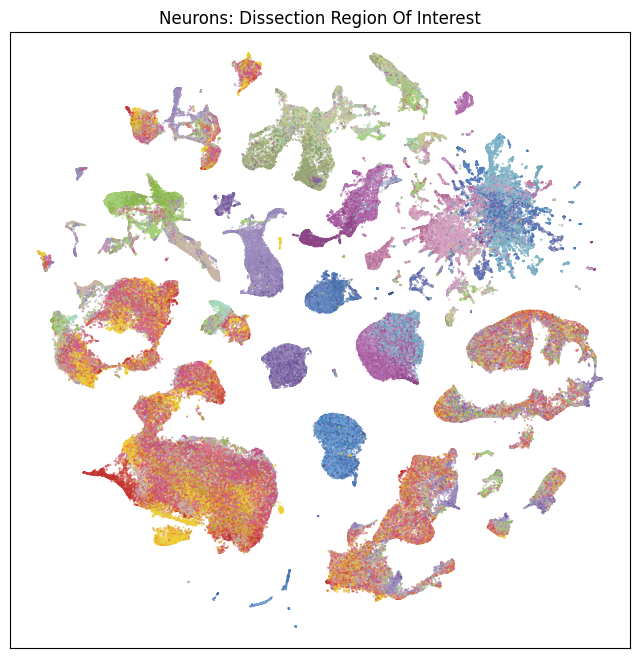
We define a small helper function plot umap to visualize the cells on the UMAP. In this example will will plot associated cell information colorized by: dissection region of interest, neurotransmitter identity, cell supercluster, cluster, and subcluster. For ease of demostration, we do a simple subsampling of the cells by a factor of 10 to reduce processing time.
def plot_umap(xx, yy, cc=None, val=None, fig_width=8, fig_height=8, cmap=None):

    fig, ax = plt.subplots()
    fig.set_size_inches(fig_width, fig_height)

    if cmap is not None:
        plt.scatter(xx, yy, s=0.5, c=val, marker='.', cmap=cmap)
    elif cc is not None:
        plt.scatter(xx, yy, s=0.5, color=cc, marker='.')

    ax.axis('equal')
    ax.set_xticks([])
    ax.set_yticks([])

    return fig, ax
neurons_subsampled = cell_extended[cell_extended['feature_matrix_label'] == 'WHB-10Xv3-Neurons'][::10]
non_neurons_subsampled = cell_extended[cell_extended['feature_matrix_label'] == 'WHB-10Xv3-Nonneurons'][::10]
print("n neurons to plot:", len(neurons_subsampled))
print("n non-neurons to plot:", len(non_neurons_subsampled))
n neurons to plot: 303681
n non-neurons to plot: 107871
fig, ax = plot_umap(neurons_subsampled['x'], neurons_subsampled['y'], cc=neurons_subsampled['region_of_interest_color'])
res = ax.set_title("Neurons: Dissection Region Of Interest")
plt.show()
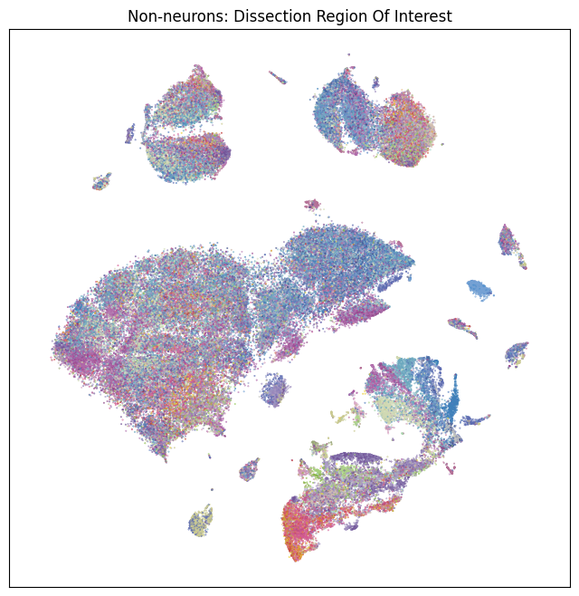
fig, ax = plot_umap(non_neurons_subsampled['x'], non_neurons_subsampled['y'], cc=non_neurons_subsampled['region_of_interest_color'])
res = ax.set_title("Non-neurons: Dissection Region Of Interest")
plt.show()
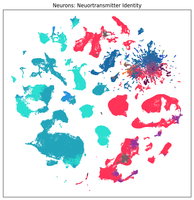
fig, ax = plot_umap(neurons_subsampled['x'], neurons_subsampled['y'], cc=neurons_subsampled['neurotransmitter_color'])
res = ax.set_title("Neurons: Neuortransmitter Identity")
plt.show()
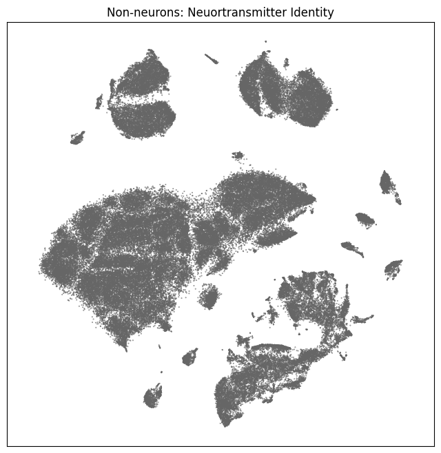
fig, ax = plot_umap(non_neurons_subsampled['x'], non_neurons_subsampled['y'], cc=non_neurons_subsampled['neurotransmitter_color'])
res = ax.set_title("Non-neurons: Neuortransmitter Identity")
plt.show()
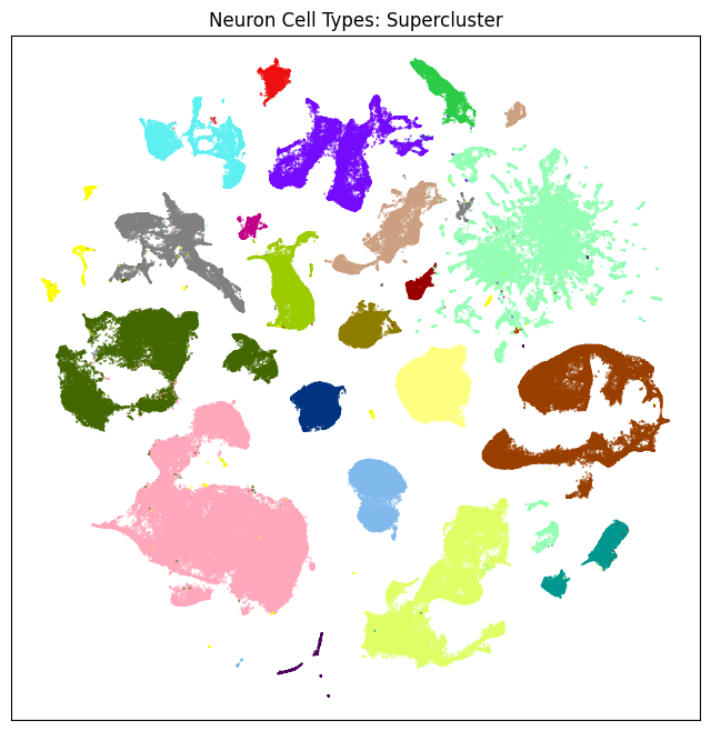
fig, ax = plot_umap(neurons_subsampled['x'], neurons_subsampled['y'], cc=neurons_subsampled['supercluster_color'])
res = ax.set_title("Neuron Cell Types: Supercluster")
plt.show()
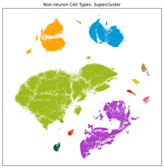
fig, ax = plot_umap(non_neurons_subsampled['x'], non_neurons_subsampled['y'], cc=non_neurons_subsampled['supercluster_color'])
res = ax.set_title("Non-neuron Cell Types: Supercluster")
plt.show()
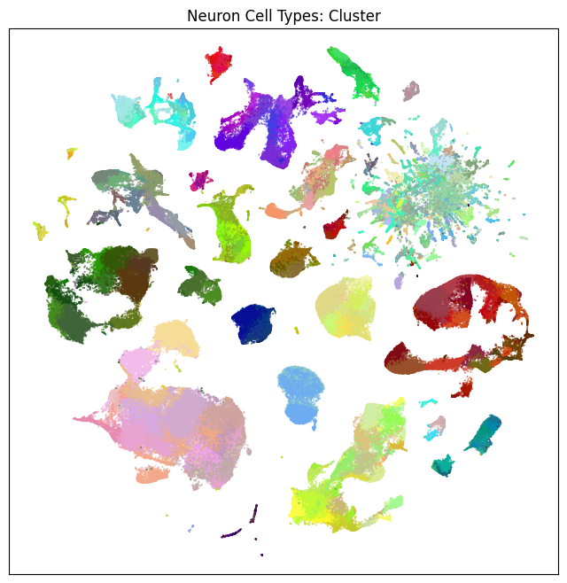
fig, ax = plot_umap(neurons_subsampled['x'], neurons_subsampled['y'], cc=neurons_subsampled['cluster_color'])
res = ax.set_title("Neuron Cell Types: Cluster")
plt.show()
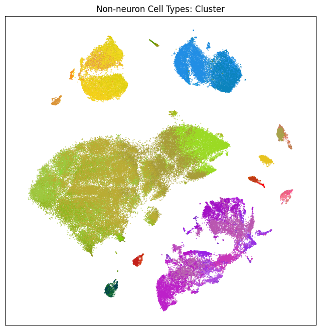
fig, ax = plot_umap(non_neurons_subsampled['x'], non_neurons_subsampled['y'], cc=non_neurons_subsampled['cluster_color'])
res = ax.set_title("Non-neuron Cell Types: Cluster")
plt.show()
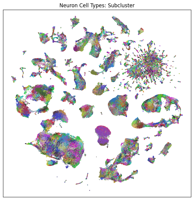
fig, ax = plot_umap(neurons_subsampled['x'], neurons_subsampled['y'], cc=neurons_subsampled['subcluster_color'])
res = ax.set_title("Neuron Cell Types: Subcluster")
plt.show()
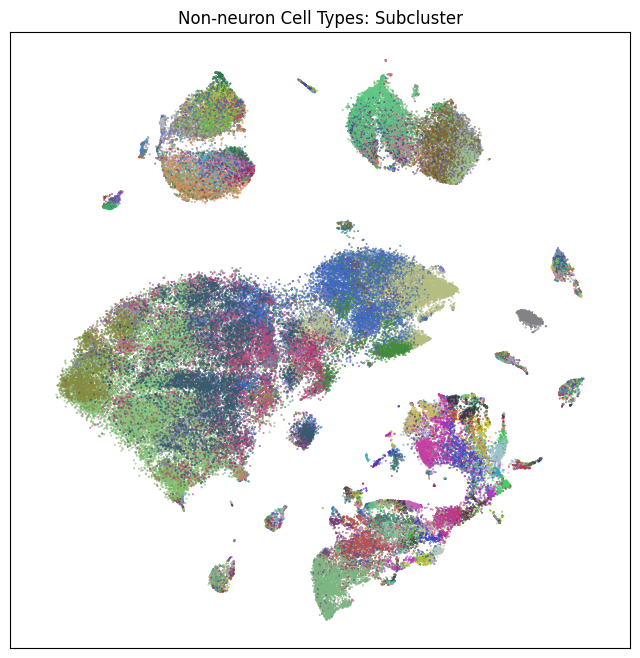
fig, ax = plot_umap(non_neurons_subsampled['x'], non_neurons_subsampled['y'], cc=non_neurons_subsampled['subcluster_color'])
res = ax.set_title("Non-neuron Cell Types: Subcluster")
plt.show()
In part 2 we’ll focus on gene data including using the UMAP to plot gene expression locations in the different clusterings.