MERFISH whole mouse brain spatial transcriptomics (Xiaowei Zhuang)#
A collection of in situ, spatially resolved transcriptomic profiles of individual cells in the whole mouse brain by multiplexed error-robust fluorescence in situ hybridization (MERFISH) consisting of ~9 million cells using a 1122 gene panel. We performed MERFISH imaging on 245 coronal and sagittal sections from four animal, obtained 9.3 million segmented cells that passed quality control, and integrated the MERFISH data from the four animals with the scRNA-seq data from the Allen Institute to classify cells. We applied a series of filters to select a subset of cells to be visualized on the ABC atlas. We first removed six fractured tissue slices and 9.1 million cells remained after this step. Then we aligned the spatial coordinates of the cells to the Allen-CCF-2020. For coronal slices that can be registered to the CCF, we used the CCF coordinates to define the coordinates of the center point of the midline and removed cells that substantially passed the midline in the other hemisphere (which has not been registered to the CCF). For the sagittal slices that can be registered to the CCF, we used the CCF coordinates to define the coordinates of the center point of the tissue and removed cells that substantially passed the posterior edge (which has not been registered to the CCF). For the 31 anterior and posterior coronal slices and 3 lateral sagittal slices that cannot be registered to the CCF, we manually aligned and oriented the slices. The x, y coordinates are experimentally measured coordinates after rotating and aligning the tissue slices to the CCF, and the z coordinates are estimated position of each tissue slice in the 3D Allen-CCF 2020 space along the slicing axis based on either the registration results (for slices that can be registered to CCF) or positions of the slices measured during tissue sectioning (for the slices that cannot be registered). The z position is set to zero when the estimated position becomes zero or negative. 8.4 million cells remained after this step. The cell-by-gene matrix of the 8.4 millions cells can be downloaded from the AWS bucket of this animal. We then filtered the cells by cell-classification (label transfer) confidence scores calculated during MERFISH-scRNAseq data integration. 7.0 million cells passed the confidence score threshold for cell subclass label transfer and 5.8 million cells further passed the confidence score threshold for cell cluster label transfer. These 5.8 million cells are included in the cell metadata file that can be downloaded from the the AWS bucket and are displayed on the ABC Atlas. The CCF coordinates of the 5.4 million cells that were registered to the 3D Allen-CCF can be downloaded from the CCF coordinate files in the AWB bucket. The collection spans four mouse specimens (2 coronal sets and 2 sagittal sets). Cells are mapped to the whole mouse brain taxonomy (WMB-taxonomy) and Allen Common Coordinate Framework (Allen-CCF-2020). Refer to Zhang et al, 2023 for more details.
import pandas as pd
from pathlib import Path
import numpy as np
import anndata
import time
import matplotlib.pyplot as plt

from abc_atlas_access.abc_atlas_cache.abc_project_cache import AbcProjectCache
We will interact with the data using the AbcProjectCache. This cache object tracks which data has been downloaded and serves the path to the requsted data on disk. For metadata, the cache can also directly serve a up a Pandas Dataframe. See the getting_started notebook for more details on using the cache including installing it if it has not already been.
Change the download_base variable to where you have downloaded the data in your system.
download_base = Path('../../data/abc_atlas')
abc_cache = AbcProjectCache.from_cache_dir(download_base)

abc_cache.current_manifest
'releases/20250531/manifest.json'
datasets = ['Zhuang-ABCA-1', 'Zhuang-ABCA-2', 'Zhuang-ABCA-3', 'Zhuang-ABCA-4']
example_section = {'Zhuang-ABCA-1': 'Zhuang-ABCA-1.079',
                   'Zhuang-ABCA-2': 'Zhuang-ABCA-2.037',
                   'Zhuang-ABCA-3': 'Zhuang-ABCA-3.010',
                   'Zhuang-ABCA-4': 'Zhuang-ABCA-4.002'}
Data overview#
Cell metadata#
Essential cell metadata is stored as a dataframe. Each row represents one cell indexed by a cell label.
Each cell is associated with a brain section label, donor label, donor genotype, donor sex and matrix_prefix identifying which data package this cell is part of. Each cell also has a set of x, y, z coordinates generated by rotating each section so that it is upright with midline approximatedly in the middle of the frame.
Each cell is mapped to the whole mouse brain taxonomy resulting in the assignment of a cluster alias and confidence scores.
cell = {}

for d in datasets :

    cell[d] = abc_cache.get_metadata_dataframe(
        directory=d,
        file_name='cell_metadata',
        dtype={"cell_label": str}
    )
    cell[d].set_index('cell_label', inplace=True)

    sdf = cell[d].groupby('brain_section_label')

    print(d,":","Number of cells = ", len(cell[d]), ", ", "Number of sections =", len(sdf))
Zhuang-ABCA-1 : Number of cells =  2846908 ,  Number of sections = 147
Zhuang-ABCA-2 : Number of cells =  1227408 ,  Number of sections = 66
Zhuang-ABCA-3 : Number of cells =  1585843 ,  Number of sections = 23
Zhuang-ABCA-4 : Number of cells =  162578 ,  Number of sections = 3
cell[datasets[0]]
| brain_section_label | feature_matrix_label | donor_label | donor_genotype | donor_sex | cluster_alias | x | y | z | subclass_confidence_score | cluster_confidence_score | high_quality_transfer | abc_sample_id | |
|---|---|---|---|---|---|---|---|---|---|---|---|---|---|
| cell_label | |||||||||||||
| 182941331246012878296807398333956011710 | Zhuang-ABCA-1.089 | Zhuang-ABCA-1 | Zhuang-ABCA-1 | wt/wt | F | 704 | 0.682522 | 3.366483 | 7.829530 | 0.969933 | 0.718088 | True | 79bda012-4dd4-43d7-8f66-1f29997f6780 |
| 221260934538535633595532020856387724686 | Zhuang-ABCA-1.089 | Zhuang-ABCA-1 | Zhuang-ABCA-1 | wt/wt | F | 5243 | 0.667690 | 3.442241 | 7.829530 | 0.850554 | 0.850554 | True | 2f0b3159-2766-4f9e-a8cd-8dd16bae05fa |
| 22228792606814781533240955623030943708 | Zhuang-ABCA-1.089 | Zhuang-ABCA-1 | Zhuang-ABCA-1 | wt/wt | F | 14939 | 0.638731 | 3.474328 | 7.829530 | 0.888285 | 0.649581 | True | fe1f5f73-5afb-4e51-b4f0-cf6690257086 |
| 272043042552227961220474294517855477150 | Zhuang-ABCA-1.089 | Zhuang-ABCA-1 | Zhuang-ABCA-1 | wt/wt | F | 14939 | 0.653425 | 3.433218 | 7.829530 | 0.900000 | 0.607080 | True | a13e1c1c-9828-4d3b-9aae-e2ab055a39ad |
| 110116287883089187971185374239350249328 | Zhuang-ABCA-1.089 | Zhuang-ABCA-1 | Zhuang-ABCA-1 | wt/wt | F | 5254 | 0.623896 | 3.513574 | 7.829530 | 0.999978 | 0.689511 | True | add02bc8-456b-486c-9f13-db578c62cc5a |
| ... | ... | ... | ... | ... | ... | ... | ... | ... | ... | ... | ... | ... | ... |
| 94310525370042131911495836073267655162 | Zhuang-ABCA-1.110 | Zhuang-ABCA-1 | Zhuang-ABCA-1 | wt/wt | F | 5255 | 0.997247 | 3.823236 | 9.717769 | 0.971385 | 0.943456 | True | 3e178fe9-3440-4cf1-ab79-2192d25e3d02 |
| 298798481479578578007190103666214714353 | Zhuang-ABCA-1.110 | Zhuang-ABCA-1 | Zhuang-ABCA-1 | wt/wt | F | 14939 | 1.043871 | 3.706231 | 9.717769 | 0.956377 | 0.905493 | True | 22cfcaf3-0c26-41b7-ab14-f76398fd18a4 |
| 330756942354980576352210203729462562749 | Zhuang-ABCA-1.110 | Zhuang-ABCA-1 | Zhuang-ABCA-1 | wt/wt | F | 5261 | 1.037680 | 3.759890 | 9.717769 | 0.811520 | 0.788901 | True | bc4eb252-c3fd-4ba0-9739-70eff08b29fe |
| 47305871059582831548494138048361484565 | Zhuang-ABCA-1.110 | Zhuang-ABCA-1 | Zhuang-ABCA-1 | wt/wt | F | 5252 | 1.044169 | 3.758463 | 9.717769 | 0.991924 | 0.634152 | True | f450f6fa-667b-40bf-a865-000131b57d2c |
| 64578198410898899234789748167671783948 | Zhuang-ABCA-1.110 | Zhuang-ABCA-1 | Zhuang-ABCA-1 | wt/wt | F | 5263 | 1.042301 | 3.589421 | 9.717769 | 0.889413 | 0.645770 | True | 11b45e69-80fe-4cd7-9480-ce3a04a9b1c5 |
2846908 rows × 13 columns
Cluster annotation#
Read in the pivot table from the “cluster annotation tutorial” to associate each cell with terms at each cell type classification level and the corresponding color.
cluster_details = abc_cache.get_metadata_dataframe(
    directory='WMB-taxonomy',
    file_name='cluster_to_cluster_annotation_membership_pivoted',
    keep_default_na=False
)
cluster_details.set_index('cluster_alias', inplace=True)

cluster_colors = abc_cache.get_metadata_dataframe(
    directory='WMB-taxonomy',
    file_name='cluster_to_cluster_annotation_membership_color',
)
cluster_colors.set_index('cluster_alias', inplace=True)
cluster_details
| neurotransmitter | class | subclass | supertype | cluster | |
|---|---|---|---|---|---|
| cluster_alias | |||||
| 1 | Glut | 01 IT-ET Glut | 018 L2 IT PPP-APr Glut | 0082 L2 IT PPP-APr Glut_3 | 0326 L2 IT PPP-APr Glut_3 |
| 2 | Glut | 01 IT-ET Glut | 018 L2 IT PPP-APr Glut | 0082 L2 IT PPP-APr Glut_3 | 0327 L2 IT PPP-APr Glut_3 |
| 3 | Glut | 01 IT-ET Glut | 018 L2 IT PPP-APr Glut | 0081 L2 IT PPP-APr Glut_2 | 0322 L2 IT PPP-APr Glut_2 |
| 4 | Glut | 01 IT-ET Glut | 018 L2 IT PPP-APr Glut | 0081 L2 IT PPP-APr Glut_2 | 0323 L2 IT PPP-APr Glut_2 |
| 5 | Glut | 01 IT-ET Glut | 018 L2 IT PPP-APr Glut | 0081 L2 IT PPP-APr Glut_2 | 0325 L2 IT PPP-APr Glut_2 |
| ... | ... | ... | ... | ... | ... |
| 34368 | GABA-Glyc | 27 MY GABA | 288 MDRN Hoxb5 Ebf2 Gly-Gaba | 1102 MDRN Hoxb5 Ebf2 Gly-Gaba_1 | 4955 MDRN Hoxb5 Ebf2 Gly-Gaba_1 |
| 34372 | GABA-Glyc | 27 MY GABA | 285 MY Lhx1 Gly-Gaba | 1091 MY Lhx1 Gly-Gaba_3 | 4901 MY Lhx1 Gly-Gaba_3 |
| 34374 | GABA-Glyc | 27 MY GABA | 285 MY Lhx1 Gly-Gaba | 1091 MY Lhx1 Gly-Gaba_3 | 4902 MY Lhx1 Gly-Gaba_3 |
| 34376 | GABA-Glyc | 27 MY GABA | 285 MY Lhx1 Gly-Gaba | 1091 MY Lhx1 Gly-Gaba_3 | 4903 MY Lhx1 Gly-Gaba_3 |
| 34380 | GABA-Glyc | 27 MY GABA | 285 MY Lhx1 Gly-Gaba | 1095 MY Lhx1 Gly-Gaba_7 | 4924 MY Lhx1 Gly-Gaba_7 |
5322 rows × 5 columns
cluster_colors
| neurotransmitter_color | class_color | subclass_color | supertype_color | cluster_color | |
|---|---|---|---|---|---|
| cluster_alias | |||||
| 1 | #2B93DF | #FA0087 | #0F6632 | #266DFF | #64661F |
| 2 | #2B93DF | #FA0087 | #0F6632 | #266DFF | #CCA73D |
| 3 | #2B93DF | #FA0087 | #0F6632 | #002BCC | #99000D |
| 4 | #2B93DF | #FA0087 | #0F6632 | #002BCC | #5C8899 |
| 5 | #2B93DF | #FA0087 | #0F6632 | #002BCC | #473D66 |
| ... | ... | ... | ... | ... | ... |
| 34368 | #820e57 | #0096C7 | #660038 | #5CCCA4 | #500099 |
| 34372 | #820e57 | #0096C7 | #f20985 | #976df9 | #0F6627 |
| 34374 | #820e57 | #0096C7 | #f20985 | #976df9 | #2E4799 |
| 34376 | #820e57 | #0096C7 | #f20985 | #976df9 | #15FF00 |
| 34380 | #820e57 | #0096C7 | #f20985 | #FF2B26 | #459988 |
5322 rows × 5 columns
cell_extended = {}

for d in datasets :
    cell_extended[d] = cell[d].join(cluster_details, on='cluster_alias')
    cell_extended[d] = cell_extended[d].join(cluster_colors, on='cluster_alias')
cell_extended[datasets[0]]
| brain_section_label | feature_matrix_label | donor_label | donor_genotype | donor_sex | cluster_alias | x | y | z | subclass_confidence_score | ... | neurotransmitter | class | subclass | supertype | cluster | neurotransmitter_color | class_color | subclass_color | supertype_color | cluster_color | |
|---|---|---|---|---|---|---|---|---|---|---|---|---|---|---|---|---|---|---|---|---|---|
| cell_label | |||||||||||||||||||||
| 182941331246012878296807398333956011710 | Zhuang-ABCA-1.089 | Zhuang-ABCA-1 | Zhuang-ABCA-1 | wt/wt | F | 704 | 0.682522 | 3.366483 | 7.829530 | 0.969933 | ... | GABA | 06 CTX-CGE GABA | 049 Lamp5 Gaba | 0199 Lamp5 Gaba_1 | 0709 Lamp5 Gaba_1 | #FF3358 | #CCFF33 | #FF764D | #DC00FF | #998900 |
| 221260934538535633595532020856387724686 | Zhuang-ABCA-1.089 | Zhuang-ABCA-1 | Zhuang-ABCA-1 | wt/wt | F | 5243 | 0.667690 | 3.442241 | 7.829530 | 0.850554 | ... | 33 Vascular | 331 Peri NN | 1191 Peri NN_1 | 5304 Peri NN_1 | #666666 | #858881 | #82992E | #2F00CC | #BB1FCC | |
| 22228792606814781533240955623030943708 | Zhuang-ABCA-1.089 | Zhuang-ABCA-1 | Zhuang-ABCA-1 | wt/wt | F | 14939 | 0.638731 | 3.474328 | 7.829530 | 0.888285 | ... | 30 Astro-Epen | 319 Astro-TE NN | 1163 Astro-TE NN_3 | 5225 Astro-TE NN_3 | #666666 | #594a26 | #3DCCB1 | #a8afa5 | #551799 | |
| 272043042552227961220474294517855477150 | Zhuang-ABCA-1.089 | Zhuang-ABCA-1 | Zhuang-ABCA-1 | wt/wt | F | 14939 | 0.653425 | 3.433218 | 7.829530 | 0.900000 | ... | 30 Astro-Epen | 319 Astro-TE NN | 1163 Astro-TE NN_3 | 5225 Astro-TE NN_3 | #666666 | #594a26 | #3DCCB1 | #a8afa5 | #551799 | |
| 110116287883089187971185374239350249328 | Zhuang-ABCA-1.089 | Zhuang-ABCA-1 | Zhuang-ABCA-1 | wt/wt | F | 5254 | 0.623896 | 3.513574 | 7.829530 | 0.999978 | ... | 33 Vascular | 333 Endo NN | 1193 Endo NN_1 | 5310 Endo NN_1 | #666666 | #858881 | #994567 | #00992A | #FFB473 | |
| ... | ... | ... | ... | ... | ... | ... | ... | ... | ... | ... | ... | ... | ... | ... | ... | ... | ... | ... | ... | ... | ... |
| 94310525370042131911495836073267655162 | Zhuang-ABCA-1.110 | Zhuang-ABCA-1 | Zhuang-ABCA-1 | wt/wt | F | 5255 | 0.997247 | 3.823236 | 9.717769 | 0.971385 | ... | 33 Vascular | 333 Endo NN | 1193 Endo NN_1 | 5311 Endo NN_1 | #666666 | #858881 | #994567 | #00992A | #CC3D76 | |
| 298798481479578578007190103666214714353 | Zhuang-ABCA-1.110 | Zhuang-ABCA-1 | Zhuang-ABCA-1 | wt/wt | F | 14939 | 1.043871 | 3.706231 | 9.717769 | 0.956377 | ... | 30 Astro-Epen | 319 Astro-TE NN | 1163 Astro-TE NN_3 | 5225 Astro-TE NN_3 | #666666 | #594a26 | #3DCCB1 | #a8afa5 | #551799 | |
| 330756942354980576352210203729462562749 | Zhuang-ABCA-1.110 | Zhuang-ABCA-1 | Zhuang-ABCA-1 | wt/wt | F | 5261 | 1.037680 | 3.759890 | 9.717769 | 0.811520 | ... | 33 Vascular | 330 VLMC NN | 1188 VLMC NN_2 | 5301 VLMC NN_2 | #666666 | #858881 | #653D66 | #4D5CFF | #79CC5C | |
| 47305871059582831548494138048361484565 | Zhuang-ABCA-1.110 | Zhuang-ABCA-1 | Zhuang-ABCA-1 | wt/wt | F | 5252 | 1.044169 | 3.758463 | 9.717769 | 0.991924 | ... | 33 Vascular | 333 Endo NN | 1193 Endo NN_1 | 5309 Endo NN_1 | #666666 | #858881 | #994567 | #00992A | #5C9994 | |
| 64578198410898899234789748167671783948 | Zhuang-ABCA-1.110 | Zhuang-ABCA-1 | Zhuang-ABCA-1 | wt/wt | F | 5263 | 1.042301 | 3.589421 | 9.717769 | 0.889413 | ... | 33 Vascular | 330 VLMC NN | 1187 VLMC NN_1 | 5298 VLMC NN_1 | #666666 | #858881 | #653D66 | #66391F | #3B9900 |
2846908 rows × 23 columns
The cell_extended dataframes are available in their respective Zhuang-ABCA-[1,2,3,4] directories as cell_metadata_with_cluster_annotation.
Gene panel#
All 4 datasets shares the same 1122 gene panel selected to enable faciliate the mapping to transcriptomically defined cell types taxonomies. Each gene is uniquely identifier by an Ensembl ID. It is best practice to gene identifier to for tracking and data interchange as gene symbols are not unique and can change over time.
Each row of the gene dataframe has Ensembl gene identifier, a gene symbol and name.
gene = abc_cache.get_metadata_dataframe(directory=datasets[0],
                                        file_name='gene')
gene.set_index('gene_identifier', inplace=True)
print("Number of genes = ", len(gene))
gene.head(5)
Number of genes = 1122
| gene_symbol | name | mapped_ncbi_identifier | |
|---|---|---|---|
| gene_identifier | |||
| ENSMUSG00000024798 | Htr7 | 5-hydroxytryptamine (serotonin) receptor 7 | NCBIGene:15566 |
| ENSMUSG00000042385 | Gzmk | granzyme K | NCBIGene:14945 |
| ENSMUSG00000036198 | Arhgap36 | Rho GTPase activating protein 36 | NCBIGene:75404 |
| ENSMUSG00000028780 | Sema3c | sema domain, immunoglobulin domain (Ig), short... | NCBIGene:20348 |
| ENSMUSG00000015843 | Rxrg | retinoid X receptor gamma | NCBIGene:20183 |
Gene expression matrix#
Expression values for all sections are stored in an anndata h5ad format per brain with minimal metadata. There are two h5ad files one storing the raw counts and the other log normalization of it. In this next section, we provide example code on how to open the file and connect with the rich cell level metadata discussed above.
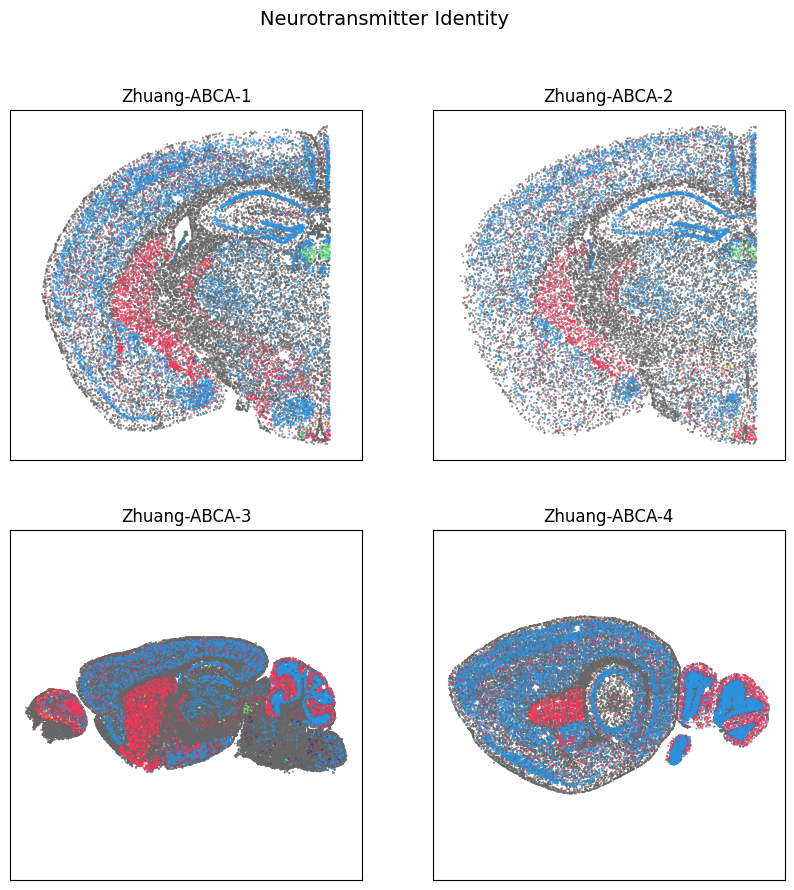
We define a small helper function plot sections to visualize the cells in anatomical context colorized by: neurotransmitter identity, cell types division, class and subclass.
def subplot_section(ax, xx, yy, cc = None, val = None, cmap = None) :

    if cmap is not None :
        ax.scatter(xx, yy, s=0.5, c=val, marker='.', cmap=cmap)
    elif cc is not None :
        ax.scatter(xx, yy, s=0.5, color=cc, marker='.')
    ax.set_ylim(11, 0)
    ax.set_xlim(0, 11)
    ax.axis('equal')
    ax.set_xticks([])
    ax.set_yticks([])
def plot_sections(cell_extended, example_section, cc = None, val = None, fig_width = 10, fig_height = 10, cmap = None) :

    fig, ax = plt.subplots(2, 2)
    fig.set_size_inches(fig_width, fig_height)

    for i, d in enumerate(cell_extended):

        pred = (cell_extended[d]['brain_section_label'] == example_section[d])
        section = cell_extended[d][pred]

        if cmap is not None :
            subplot_section( ax.flat[i], section['x'], section['y'], val=section[val], cmap=cmap)
        elif cc is not None :
            subplot_section( ax.flat[i], section['x'], section['y'], section[cc])

        ax.flat[i].set_title(d)

    return fig, ax
fig, ax = plot_sections(cell_extended, example_section, 'neurotransmitter_color')
res = fig.suptitle('Neurotransmitter Identity', fontsize=14)
plt.show()
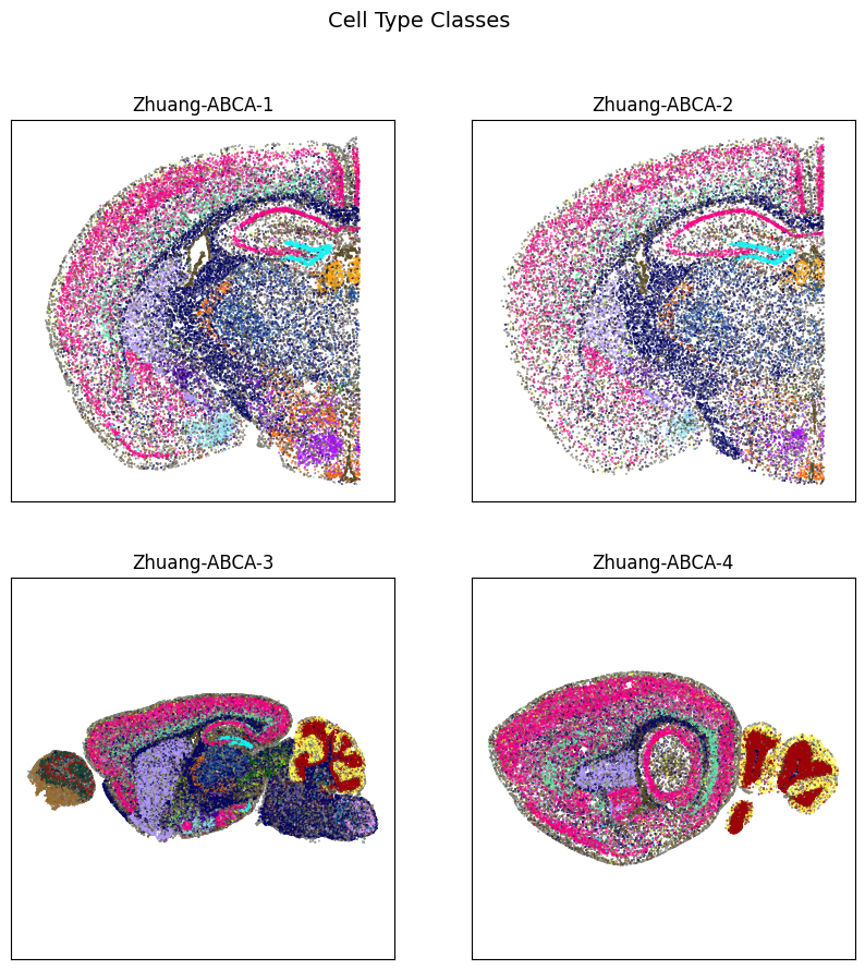
fig, ax = plot_sections(cell_extended, example_section, 'class_color')
res = fig.suptitle('Cell Type Classes', fontsize=14)
plt.show()
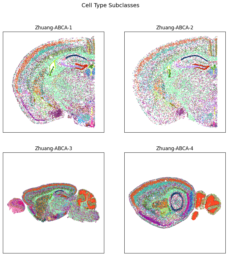
fig, ax = plot_sections(cell_extended, example_section, 'subclass_color')
res = fig.suptitle('Cell Type Subclasses', fontsize=14)
plt.show()
Example use case#
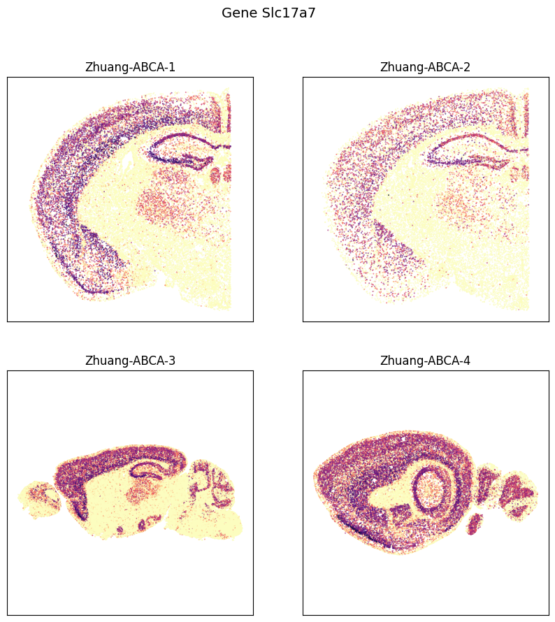
In this section, we visualize the expression of nine canonical neurotransmitter transporter genes. To support these use cases, we will create a smaller submatrix (all cells and 9 genes) that read it into dataframe. Note this operation takes around 2-5 minutes.
gnames = ['Slc17a7', 'Slc17a6', 'Slc17a8', 'Slc32a1', 'Slc6a5', 'Slc6a3', 'Slc6a4']
pred = [x in gnames for x in gene.gene_symbol]
gene_filtered = gene[pred]
gene_filtered
| gene_symbol | name | mapped_ncbi_identifier | |
|---|---|---|---|
| gene_identifier | |||
| ENSMUSG00000019935 | Slc17a8 | solute carrier family 17 (sodium-dependent ino... | NCBIGene:216227 |
| ENSMUSG00000021609 | Slc6a3 | solute carrier family 6 (neurotransmitter tran... | NCBIGene:13162 |
| ENSMUSG00000037771 | Slc32a1 | solute carrier family 32 (GABA vesicular trans... | NCBIGene:22348 |
| ENSMUSG00000039728 | Slc6a5 | solute carrier family 6 (neurotransmitter tran... | NCBIGene:104245 |
| ENSMUSG00000070570 | Slc17a7 | solute carrier family 17 (sodium-dependent ino... | NCBIGene:72961 |
| ENSMUSG00000020838 | Slc6a4 | solute carrier family 6 (neurotransmitter tran... | NCBIGene:15567 |
| ENSMUSG00000030500 | Slc17a6 | solute carrier family 17 (sodium-dependent ino... | NCBIGene:140919 |
abc_cache.list_expression_matrix_files('Zhuang-ABCA-2')
['Zhuang-ABCA-2/log2', 'Zhuang-ABCA-2/raw']
cell_expression = {}

for d in datasets:
    file = abc_cache.get_file_path(directory=d, file_name=f"{d}/log2")

    adata = anndata.read_h5ad(file, backed='r')

    start = time.process_time()
    gdata = adata[:, gene_filtered.index].to_df()
    gdata.columns = gene_filtered.gene_symbol
    cell_expression[d] = cell_extended[d].join(gdata)

    print(d,"-","time taken: ", time.process_time() - start)

    adata.file.close()
    del adata
Zhuang-ABCA-1 - time taken:  19.86417
Zhuang-ABCA-2 - time taken:  9.300148999999998
Zhuang-ABCA-3 - time taken:  9.771411999999998
Zhuang-ABCA-4-log2.h5ad: 100%|██████████| 107M/107M [04:16<00:00, 416kMB/s]
Zhuang-ABCA-4 - time taken: 1.0832089999999965
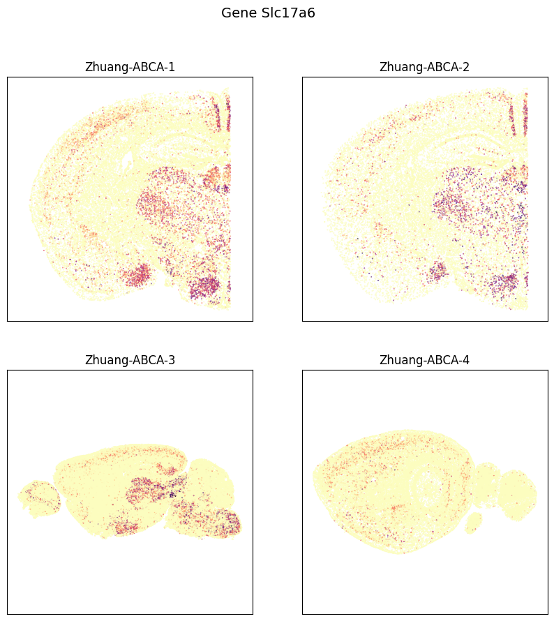
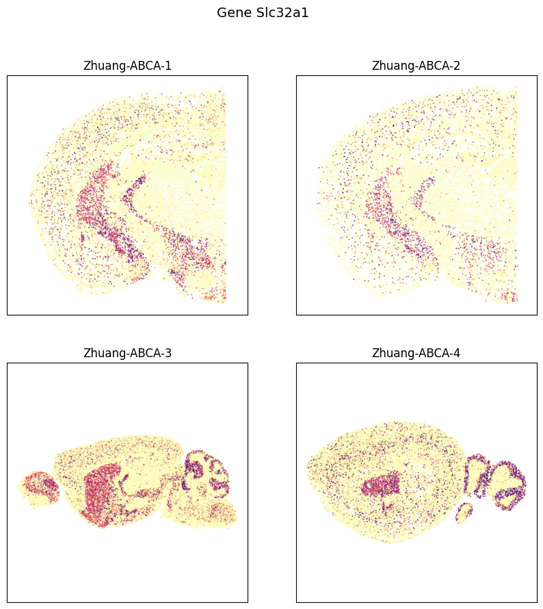
Visualize genes Slc17a7, Slc17a6, Slc32a1 for an example section from each brain
fig, ax = plot_sections(cell_expression, example_section, val='Slc17a7', cmap=plt.cm.magma_r)
res = fig.suptitle('Gene Slc17a7', fontsize=14)
plt.show()
fig, ax = plot_sections(cell_expression, example_section, val='Slc17a6', cmap=plt.cm.magma_r)
res = fig.suptitle('Gene Slc17a6', fontsize=14)
plt.show()
fig, ax = plot_sections(cell_expression, example_section, val='Slc32a1', cmap=plt.cm.magma_r)
res = fig.suptitle('Gene Slc32a1', fontsize=14)
plt.show()
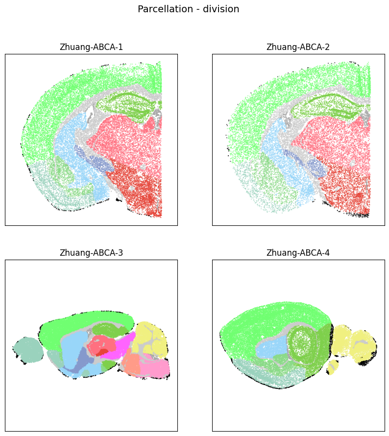
CCF registration and parcellation annotation#
Each brain specimen has been registered to Allen CCFv3 atlas, resulting in an x, y, z coordinates and parcellation_index for each cell.
ccf_coordinates = {}

for d in datasets :

    ccf_coordinates[d] = abc_cache.get_metadata_dataframe(directory=f"{d}-CCF", file_name='ccf_coordinates')
    ccf_coordinates[d].set_index('cell_label', inplace=True)
    ccf_coordinates[d].rename(columns={'x': 'x_ccf',
                                       'y': 'y_ccf',
                                       'z': 'z_ccf'},
                              inplace=True)

    cell_extended[d] = cell_extended[d].join(ccf_coordinates[d], how='inner')
ccf_coordinates.csv: 100%|██████████| 221M/221M [00:16<00:00, 13.1MMB/s]
ccf_coordinates.csv: 100%|██████████| 89.1M/89.1M [00:06<00:00, 13.6MMB/s]
ccf_coordinates.csv: 100%|██████████| 132M/132M [00:09<00:00, 13.3MMB/s]
ccf_coordinates.csv: 100%|██████████| 13.8M/13.8M [00:01<00:00, 11.8MMB/s]
ccf_coordinates[datasets[0]]
| x_ccf | y_ccf | z_ccf | parcellation_index | |
|---|---|---|---|---|
| cell_label | ||||
| 182941331246012878296807398333956011710 | 7.902190 | 3.048426 | 0.582962 | 0 |
| 221260934538535633595532020856387724686 | 7.906513 | 3.145200 | 0.577602 | 0 |
| 22228792606814781533240955623030943708 | 7.906110 | 3.182761 | 0.553731 | 0 |
| 272043042552227961220474294517855477150 | 7.904627 | 3.131808 | 0.563525 | 0 |
| 110116287883089187971185374239350249328 | 7.907236 | 3.230647 | 0.543048 | 0 |
| ... | ... | ... | ... | ... |
| 94310525370042131911495836073267655162 | 9.681244 | 4.453979 | 0.852027 | 0 |
| 298798481479578578007190103666214714353 | 9.676999 | 4.291647 | 0.899531 | 1109 |
| 330756942354980576352210203729462562749 | 9.678760 | 4.363282 | 0.894082 | 1109 |
| 47305871059582831548494138048361484565 | 9.678641 | 4.360346 | 0.901195 | 1109 |
| 64578198410898899234789748167671783948 | 9.673530 | 4.138034 | 0.897311 | 1109 |
2616328 rows × 4 columns
Read in the pivot table from the “parcellation annotation tutorial” to associate each cell with terms at each anatomical parcellation level and the corresponding color.
parcellation_annotation = abc_cache.get_metadata_dataframe(directory="Allen-CCF-2020",
                                                           file_name='parcellation_to_parcellation_term_membership_acronym')
parcellation_annotation.set_index('parcellation_index', inplace=True)
parcellation_annotation.columns = ['parcellation_%s'% x for x in  parcellation_annotation.columns]

parcellation_color = abc_cache.get_metadata_dataframe(directory="Allen-CCF-2020",
                                                      file_name='parcellation_to_parcellation_term_membership_color')
parcellation_color.set_index('parcellation_index', inplace=True)
parcellation_color.columns = ['parcellation_%s'% x for x in  parcellation_color.columns]
for d in datasets :
    cell_extended[d] = cell_extended[d].join(parcellation_annotation, on='parcellation_index')
    cell_extended[d] = cell_extended[d].join(parcellation_color, on='parcellation_index')
fig, ax = plot_sections(cell_extended, example_section, 'parcellation_division_color')
res = fig.suptitle('Parcellation - division', fontsize=14)
plt.show()
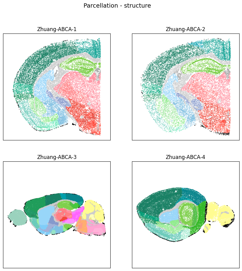
fig, ax = plot_sections(cell_extended, example_section, 'parcellation_structure_color')
res = fig.suptitle('Parcellation - structure', fontsize=14)
plt.show()
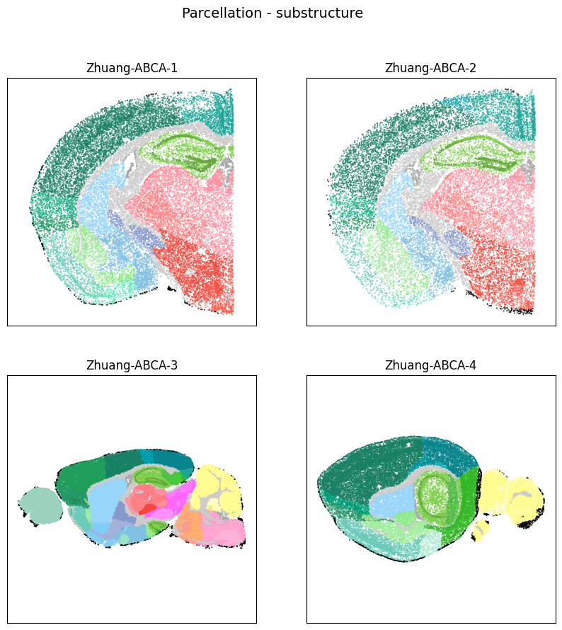
fig, ax = plot_sections(cell_extended, example_section, 'parcellation_substructure_color')
res = fig.suptitle('Parcellation - substructure', fontsize=14)
plt.show()