10x RNA-seq gene expression data (part 1)#
To efficiently handle data transfer and download, the 4 million cell 10X dataset, was subdivide into 24 expression matrices where cells are grouped by 10X chemistry (10Xv2, 10Xv3 and 10XMulti) and the broad anatomical region from where the cells were dissected from.
The purpose of this set of notebooks is to provide an overview of the data, the file organization and how to combine data and metadata through example use cases.
You need to be connected to the internet to run this notebook and have run through the getting started notebook.
import pandas as pd
from pathlib import Path
import numpy as np
import anndata
import time
import matplotlib.pyplot as plt

from abc_atlas_access.abc_atlas_cache.abc_project_cache import AbcProjectCache
We will interact with the data using the AbcProjectCache. This cache object tracks which data has been downloaded and serves the path to the requsted data on disk. For metadata, the cache can also directly serve a up a Pandas Dataframe. See the getting_started notebook for more details on using the cache including installing it if it has not already been.
Change the download_base variable to where you have downloaded the data in your system.
download_base = Path('../../data/abc_atlas')
abc_cache = AbcProjectCache.from_cache_dir(download_base)

abc_cache.current_manifest
'releases/20250531/manifest.json'
Data overview#
Cell metadata#
Essential cell metadata is stored as a dataframe. Each row represents one cell indexed by a cell label. The cell label is the concatenation of barcode and name of the sample. In this context, the sample is the barcoded cell sample that represents a single load into one port of the 10x Chromium. Note that cell barcodes are only unique within a single barcoded cell sample and that the same barcode can be reused. The barcoded cell sample label or name is unique in the database.
Each cell is associated with a library label, library method, donor label, donor genotype, donor sex, dissection *region of interest acronym”, the corresponding coarse anatomical division label and the matrix_prefix identifying which data package this cell is part of.
Further, each cell is associated with a cluster alias representing which cluster this cell is a member of and (x,y) coordinates of the all cells UMAP in Figure 1 of the manuscript.
Below, we list the metadata files we will be using in this tutorial.
abc_cache.list_metadata_files('WMB-10X')
['cell_metadata',
 'cell_metadata_with_cluster_annotation',
 'example_genes_all_cells_expression',
 'gene',
 'region_of_interest_metadata']
abc_cache.list_metadata_files('WMB-taxonomy')
['cluster',
 'cluster_annotation_term',
 'cluster_annotation_term_set',
 'cluster_annotation_term_with_counts',
 'cluster_to_cluster_annotation_membership',
 'cluster_to_cluster_annotation_membership_color',
 'cluster_to_cluster_annotation_membership_pivoted']
abc_cache.get_directory_metadata('WMB-taxonomy')
[PosixPath('/Users/chris.morrison/src/data/abc_atlas/metadata/WMB-taxonomy/20231215/cluster.csv'),
 PosixPath('/Users/chris.morrison/src/data/abc_atlas/metadata/WMB-taxonomy/20231215/cluster_annotation_term.csv'),
 PosixPath('/Users/chris.morrison/src/data/abc_atlas/metadata/WMB-taxonomy/20231215/cluster_annotation_term_set.csv'),
 PosixPath('/Users/chris.morrison/src/data/abc_atlas/metadata/WMB-taxonomy/20231215/views/cluster_annotation_term_with_counts.csv'),
 PosixPath('/Users/chris.morrison/src/data/abc_atlas/metadata/WMB-taxonomy/20231215/cluster_to_cluster_annotation_membership.csv'),
 PosixPath('/Users/chris.morrison/src/data/abc_atlas/metadata/WMB-taxonomy/20231215/views/cluster_to_cluster_annotation_membership_color.csv'),
 PosixPath('/Users/chris.morrison/src/data/abc_atlas/metadata/WMB-taxonomy/20231215/views/cluster_to_cluster_annotation_membership_pivoted.csv')]
abc_cache.list_expression_matrix_files('WMB-10Xv3')
['WMB-10Xv3-CB/log2',
 'WMB-10Xv3-CB/raw',
 'WMB-10Xv3-CTXsp/log2',
 'WMB-10Xv3-CTXsp/raw',
 'WMB-10Xv3-HPF/log2',
 'WMB-10Xv3-HPF/raw',
 'WMB-10Xv3-HY/log2',
 'WMB-10Xv3-HY/raw',
 'WMB-10Xv3-Isocortex-1/log2',
 'WMB-10Xv3-Isocortex-1/raw',
 'WMB-10Xv3-Isocortex-2/log2',
 'WMB-10Xv3-Isocortex-2/raw',
 'WMB-10Xv3-MB/log2',
 'WMB-10Xv3-MB/raw',
 'WMB-10Xv3-MY/log2',
 'WMB-10Xv3-MY/raw',
 'WMB-10Xv3-OLF/log2',
 'WMB-10Xv3-OLF/raw',
 'WMB-10Xv3-P/log2',
 'WMB-10Xv3-P/raw',
 'WMB-10Xv3-PAL/log2',
 'WMB-10Xv3-PAL/raw',
 'WMB-10Xv3-STR/log2',
 'WMB-10Xv3-STR/raw',
 'WMB-10Xv3-TH/log2',
 'WMB-10Xv3-TH/raw']
Below, we load the first of the metadata used in this tutorial. This pattern of loading metadata is repeated throughout the tutorials.
cell = abc_cache.get_metadata_dataframe(
    directory='WMB-10X',
    file_name='cell_metadata',
    dtype={'cell_label': str}
)
cell.set_index('cell_label', inplace=True)
print("Number of cells = ", len(cell))
cell.head(5)
cell_metadata.csv: 100%|██████████| 1.01G/1.01G [02:05<00:00, 8.01MMB/s]
Number of cells = 4042976
| cell_barcode | barcoded_cell_sample_label | library_label | feature_matrix_label | entity | brain_section_label | library_method | region_of_interest_acronym | donor_label | donor_genotype | donor_sex | dataset_label | x | y | cluster_alias | abc_sample_id | |
|---|---|---|---|---|---|---|---|---|---|---|---|---|---|---|---|---|
| cell_label | ||||||||||||||||
| GCGAGAAGTTAAGGGC-410_B05 | GCGAGAAGTTAAGGGC | 410_B05 | L8TX_201030_01_C12 | WMB-10Xv3-HPF | cell | NaN | 10Xv3 | RHP | Snap25-IRES2-Cre;Ai14-550850 | Ai14(RCL-tdT)/wt | F | WMB-10Xv3 | 23.146826 | -3.086639 | 1 | 484be5df-5d44-4bfe-9652-7b5bc739c211 |
| AATGGCTCAGCTCCTT-411_B06 | AATGGCTCAGCTCCTT | 411_B06 | L8TX_201029_01_E10 | WMB-10Xv3-HPF | cell | NaN | 10Xv3 | RHP | Snap25-IRES2-Cre;Ai14-550851 | Ai14(RCL-tdT)/wt | F | WMB-10Xv3 | 23.138481 | -3.022000 | 1 | 5638505d-e1e8-457f-9e5b-59e3e2302417 |
| AACACACGTTGCTTGA-410_B05 | AACACACGTTGCTTGA | 410_B05 | L8TX_201030_01_C12 | WMB-10Xv3-HPF | cell | NaN | 10Xv3 | RHP | Snap25-IRES2-Cre;Ai14-550850 | Ai14(RCL-tdT)/wt | F | WMB-10Xv3 | 23.472557 | -2.992709 | 1 | a0544e29-194f-4d34-9af4-13e7377b648f |
| CACAGATAGAGGCGGA-410_A05 | CACAGATAGAGGCGGA | 410_A05 | L8TX_201029_01_A10 | WMB-10Xv3-HPF | cell | NaN | 10Xv3 | RHP | Snap25-IRES2-Cre;Ai14-550850 | Ai14(RCL-tdT)/wt | F | WMB-10Xv3 | 23.379622 | -3.043442 | 1 | c777ac0b-77e1-4d76-bf8e-2b3d9e08b253 |
| AAAGTGAAGCATTTCG-410_B05 | AAAGTGAAGCATTTCG | 410_B05 | L8TX_201030_01_C12 | WMB-10Xv3-HPF | cell | NaN | 10Xv3 | RHP | Snap25-IRES2-Cre;Ai14-550850 | Ai14(RCL-tdT)/wt | F | WMB-10Xv3 | 23.909480 | -2.601536 | 1 | 49860925-e82b-46df-a228-fd2f97e75d39 |
We can use panadas groupby function to see how many unique items are associated for each field and list them out if the number of items is small.
def print_column_info(df):

    for c in df.columns:
        grouped = df[[c]].groupby(c).count()
        members = ''
        if len(grouped) < 30:
            members = str(list(grouped.index))
        print("Number of unique %s = %d %s" % (c, len(grouped), members))
print_column_info(cell)
Number of unique cell_barcode = 2375490
Number of unique barcoded_cell_sample_label = 819
Number of unique library_label = 819
Number of unique feature_matrix_label = 24 ['WMB-10XMulti', 'WMB-10Xv2-CTXsp', 'WMB-10Xv2-HPF', 'WMB-10Xv2-HY', 'WMB-10Xv2-Isocortex-1', 'WMB-10Xv2-Isocortex-2', 'WMB-10Xv2-Isocortex-3', 'WMB-10Xv2-Isocortex-4', 'WMB-10Xv2-MB', 'WMB-10Xv2-OLF', 'WMB-10Xv2-TH', 'WMB-10Xv3-CB', 'WMB-10Xv3-CTXsp', 'WMB-10Xv3-HPF', 'WMB-10Xv3-HY', 'WMB-10Xv3-Isocortex-1', 'WMB-10Xv3-Isocortex-2', 'WMB-10Xv3-MB', 'WMB-10Xv3-MY', 'WMB-10Xv3-OLF', 'WMB-10Xv3-P', 'WMB-10Xv3-PAL', 'WMB-10Xv3-STR', 'WMB-10Xv3-TH']
Number of unique entity = 1 ['cell']
Number of unique brain_section_label = 0 []
Number of unique library_method = 3 ['10Xv2', '10Xv3', '10xRSeq_Mult']
Number of unique region_of_interest_acronym = 29 ['ACA', 'AI', 'AUD', 'AUD-TEa-PERI-ECT', 'CB', 'CTXsp', 'ENT', 'HIP', 'HY', 'LSX', 'MB', 'MO-FRP', 'MOp', 'MY', 'OLF', 'P', 'PAL', 'PL-ILA-ORB', 'RHP', 'RSP', 'SS-GU-VISC', 'SSp', 'STRd', 'STRv', 'TEa-PERI-ECT', 'TH', 'VIS', 'VIS-PTLp', 'sAMY']
Number of unique donor_label = 345
Number of unique donor_genotype = 5 ['Ai14(RCL-tdT)/wt', 'Gad2-IRES-Cre/wt;Ai14(RCL-tdT)/wt', 'Slc32a1-IRES-Cre/wt;Ai14(RCL-tdT)/wt', 'Snap25-IRES2-Cre/wt;Ai14(RCL-tdT)/wt', 'wt/wt']
Number of unique donor_sex = 2 ['F', 'M']
Number of unique dataset_label = 3 ['WMB-10XMulti', 'WMB-10Xv2', 'WMB-10Xv3']
Number of unique x = 3992539
Number of unique y = 3992791
Number of unique cluster_alias = 5322
Number of unique abc_sample_id = 4042976
cell.groupby('dataset_label')[['x']].count()
| x | |
|---|---|
| dataset_label | |
| WMB-10XMulti | 1687 |
| WMB-10Xv2 | 1699939 |
| WMB-10Xv3 | 2341350 |
We can also bring in the pivot table from the “cluster annotation tutorial” to associate each cell with terms at each cell type classification level.
cluster_details = abc_cache.get_metadata_dataframe(
    directory='WMB-taxonomy',
    file_name='cluster_to_cluster_annotation_membership_pivoted',
    keep_default_na=False
)
cluster_details.set_index('cluster_alias', inplace=True)
cluster_details.head(5)
| neurotransmitter | class | subclass | supertype | cluster | |
|---|---|---|---|---|---|
| cluster_alias | |||||
| 1 | Glut | 01 IT-ET Glut | 018 L2 IT PPP-APr Glut | 0082 L2 IT PPP-APr Glut_3 | 0326 L2 IT PPP-APr Glut_3 |
| 2 | Glut | 01 IT-ET Glut | 018 L2 IT PPP-APr Glut | 0082 L2 IT PPP-APr Glut_3 | 0327 L2 IT PPP-APr Glut_3 |
| 3 | Glut | 01 IT-ET Glut | 018 L2 IT PPP-APr Glut | 0081 L2 IT PPP-APr Glut_2 | 0322 L2 IT PPP-APr Glut_2 |
| 4 | Glut | 01 IT-ET Glut | 018 L2 IT PPP-APr Glut | 0081 L2 IT PPP-APr Glut_2 | 0323 L2 IT PPP-APr Glut_2 |
| 5 | Glut | 01 IT-ET Glut | 018 L2 IT PPP-APr Glut | 0081 L2 IT PPP-APr Glut_2 | 0325 L2 IT PPP-APr Glut_2 |
cluster_colors = abc_cache.get_metadata_dataframe(
    directory='WMB-taxonomy',
    file_name='cluster_to_cluster_annotation_membership_color'
)
cluster_colors.set_index('cluster_alias', inplace=True)
cluster_colors.head(5)
| neurotransmitter_color | class_color | subclass_color | supertype_color | cluster_color | |
|---|---|---|---|---|---|
| cluster_alias | |||||
| 1 | #2B93DF | #FA0087 | #0F6632 | #266DFF | #64661F |
| 2 | #2B93DF | #FA0087 | #0F6632 | #266DFF | #CCA73D |
| 3 | #2B93DF | #FA0087 | #0F6632 | #002BCC | #99000D |
| 4 | #2B93DF | #FA0087 | #0F6632 | #002BCC | #5C8899 |
| 5 | #2B93DF | #FA0087 | #0F6632 | #002BCC | #473D66 |
roi = abc_cache.get_metadata_dataframe(directory='WMB-10X', file_name='region_of_interest_metadata')
roi.set_index('acronym', inplace=True)
roi.rename(columns={'order': 'region_of_interest_order',
                    'color_hex_triplet': 'region_of_interest_color'},
           inplace=True)
roi.head(5)
region_of_interest_metadata.csv: 100%|██████████| 1.40k/1.40k [00:00<00:00, 27.0kMB/s]
| label | name | region_of_interest_order | region_of_interest_color | |
|---|---|---|---|---|
| acronym | ||||
| MO-FRP | WMB-MO-FRP | Somatomotor - Frontal pole | 0 | #3DCC7C |
| MOp | WMB-MOp | Primary motor area | 1 | #179968 |
| SS-GU-VISC | WMB-SS-GU-VISC | Somatosensory/gustatory/visceral areas | 2 | #2E8599 |
| SSp | WMB-SSp | Primary somatosensory area | 3 | #5CCCCC |
| AUD | WMB-AUD | Auditory areas | 4 | #455A99 |
cell_extended = cell.join(cluster_details, on='cluster_alias')
cell_extended = cell_extended.join(cluster_colors, on='cluster_alias')
cell_extended = cell_extended.join(roi[['region_of_interest_order', 'region_of_interest_color']], on='region_of_interest_acronym')
cell_extended.head(5)
| cell_barcode | barcoded_cell_sample_label | library_label | feature_matrix_label | entity | brain_section_label | library_method | region_of_interest_acronym | donor_label | donor_genotype | ... | subclass | supertype | cluster | neurotransmitter_color | class_color | subclass_color | supertype_color | cluster_color | region_of_interest_order | region_of_interest_color | |
|---|---|---|---|---|---|---|---|---|---|---|---|---|---|---|---|---|---|---|---|---|---|
| cell_label | |||||||||||||||||||||
| GCGAGAAGTTAAGGGC-410_B05 | GCGAGAAGTTAAGGGC | 410_B05 | L8TX_201030_01_C12 | WMB-10Xv3-HPF | cell | NaN | 10Xv3 | RHP | Snap25-IRES2-Cre;Ai14-550850 | Ai14(RCL-tdT)/wt | ... | 018 L2 IT PPP-APr Glut | 0082 L2 IT PPP-APr Glut_3 | 0326 L2 IT PPP-APr Glut_3 | #2B93DF | #FA0087 | #0F6632 | #266DFF | #64661F | 15 | #CCB05C |
| AATGGCTCAGCTCCTT-411_B06 | AATGGCTCAGCTCCTT | 411_B06 | L8TX_201029_01_E10 | WMB-10Xv3-HPF | cell | NaN | 10Xv3 | RHP | Snap25-IRES2-Cre;Ai14-550851 | Ai14(RCL-tdT)/wt | ... | 018 L2 IT PPP-APr Glut | 0082 L2 IT PPP-APr Glut_3 | 0326 L2 IT PPP-APr Glut_3 | #2B93DF | #FA0087 | #0F6632 | #266DFF | #64661F | 15 | #CCB05C |
| AACACACGTTGCTTGA-410_B05 | AACACACGTTGCTTGA | 410_B05 | L8TX_201030_01_C12 | WMB-10Xv3-HPF | cell | NaN | 10Xv3 | RHP | Snap25-IRES2-Cre;Ai14-550850 | Ai14(RCL-tdT)/wt | ... | 018 L2 IT PPP-APr Glut | 0082 L2 IT PPP-APr Glut_3 | 0326 L2 IT PPP-APr Glut_3 | #2B93DF | #FA0087 | #0F6632 | #266DFF | #64661F | 15 | #CCB05C |
| CACAGATAGAGGCGGA-410_A05 | CACAGATAGAGGCGGA | 410_A05 | L8TX_201029_01_A10 | WMB-10Xv3-HPF | cell | NaN | 10Xv3 | RHP | Snap25-IRES2-Cre;Ai14-550850 | Ai14(RCL-tdT)/wt | ... | 018 L2 IT PPP-APr Glut | 0082 L2 IT PPP-APr Glut_3 | 0326 L2 IT PPP-APr Glut_3 | #2B93DF | #FA0087 | #0F6632 | #266DFF | #64661F | 15 | #CCB05C |
| AAAGTGAAGCATTTCG-410_B05 | AAAGTGAAGCATTTCG | 410_B05 | L8TX_201030_01_C12 | WMB-10Xv3-HPF | cell | NaN | 10Xv3 | RHP | Snap25-IRES2-Cre;Ai14-550850 | Ai14(RCL-tdT)/wt | ... | 018 L2 IT PPP-APr Glut | 0082 L2 IT PPP-APr Glut_3 | 0326 L2 IT PPP-APr Glut_3 | #2B93DF | #FA0087 | #0F6632 | #266DFF | #64661F | 15 | #CCB05C |
5 rows × 28 columns
print_column_info(cell_extended)
Number of unique cell_barcode = 2375490
Number of unique barcoded_cell_sample_label = 819
Number of unique library_label = 819
Number of unique feature_matrix_label = 24 ['WMB-10XMulti', 'WMB-10Xv2-CTXsp', 'WMB-10Xv2-HPF', 'WMB-10Xv2-HY', 'WMB-10Xv2-Isocortex-1', 'WMB-10Xv2-Isocortex-2', 'WMB-10Xv2-Isocortex-3', 'WMB-10Xv2-Isocortex-4', 'WMB-10Xv2-MB', 'WMB-10Xv2-OLF', 'WMB-10Xv2-TH', 'WMB-10Xv3-CB', 'WMB-10Xv3-CTXsp', 'WMB-10Xv3-HPF', 'WMB-10Xv3-HY', 'WMB-10Xv3-Isocortex-1', 'WMB-10Xv3-Isocortex-2', 'WMB-10Xv3-MB', 'WMB-10Xv3-MY', 'WMB-10Xv3-OLF', 'WMB-10Xv3-P', 'WMB-10Xv3-PAL', 'WMB-10Xv3-STR', 'WMB-10Xv3-TH']
Number of unique entity = 1 ['cell']
Number of unique brain_section_label = 0 []
Number of unique library_method = 3 ['10Xv2', '10Xv3', '10xRSeq_Mult']
Number of unique region_of_interest_acronym = 29 ['ACA', 'AI', 'AUD', 'AUD-TEa-PERI-ECT', 'CB', 'CTXsp', 'ENT', 'HIP', 'HY', 'LSX', 'MB', 'MO-FRP', 'MOp', 'MY', 'OLF', 'P', 'PAL', 'PL-ILA-ORB', 'RHP', 'RSP', 'SS-GU-VISC', 'SSp', 'STRd', 'STRv', 'TEa-PERI-ECT', 'TH', 'VIS', 'VIS-PTLp', 'sAMY']
Number of unique donor_label = 345
Number of unique donor_genotype = 5 ['Ai14(RCL-tdT)/wt', 'Gad2-IRES-Cre/wt;Ai14(RCL-tdT)/wt', 'Slc32a1-IRES-Cre/wt;Ai14(RCL-tdT)/wt', 'Snap25-IRES2-Cre/wt;Ai14(RCL-tdT)/wt', 'wt/wt']
Number of unique donor_sex = 2 ['F', 'M']
Number of unique dataset_label = 3 ['WMB-10XMulti', 'WMB-10Xv2', 'WMB-10Xv3']
Number of unique x = 3992539
Number of unique y = 3992791
Number of unique cluster_alias = 5322
Number of unique abc_sample_id = 4042976
Number of unique neurotransmitter = 10 ['', 'Chol', 'Dopa', 'GABA', 'GABA-Glyc', 'Glut', 'Glut-GABA', 'Hist', 'Nora', 'Sero']
Number of unique class = 34
Number of unique subclass = 338
Number of unique supertype = 1201
Number of unique cluster = 5322
Number of unique neurotransmitter_color = 10 ['#03EDFF', '#0a9964', '#2B93DF', '#533691', '#666666', '#73E785', '#820e57', '#FF3358', '#fcf04b', '#ff7621']
Number of unique class_color = 34
Number of unique subclass_color = 338
Number of unique supertype_color = 1201
Number of unique cluster_color = 5298
Number of unique region_of_interest_order = 29 [0, 1, 2, 3, 4, 5, 6, 7, 8, 9, 10, 11, 12, 13, 14, 15, 16, 17, 18, 19, 20, 21, 22, 23, 24, 25, 26, 27, 28]
Number of unique region_of_interest_color = 29 ['#0059CC', '#00990A', '#00FFCF', '#179968', '#26AEFF', '#2E8599', '#300099', '#341FCC', '#34CC1F', '#3DCC7C', '#455A99', '#4D58FF', '#5CCCCC', '#6F9945', '#84FF4D', '#8CCC00', '#992E6A', '#994817', '#99922E', '#9F3DCC', '#B973FF', '#CC0026', '#CC5CB0', '#CCB05C', '#E4FF26', '#FF00EF', '#FF2678', '#FF7373', '#FF8F00']
The joined table above can be written to disk be later use, however, a copy can be found in the cache as under the name ‘cell_metadata_with_cluster_annotation’.
UMAP spatial embedding#
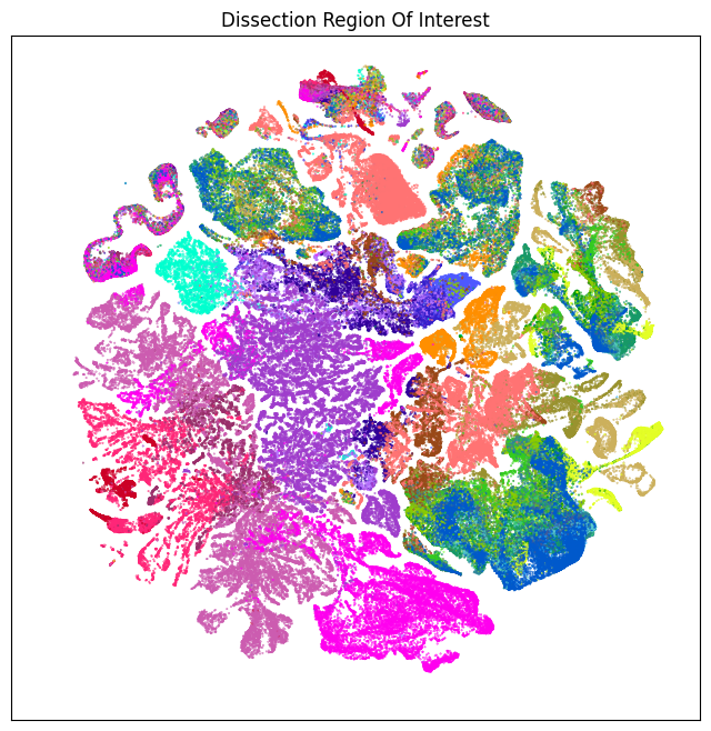
Uniform Manifold Approximation and Projection (UMAP) is a dimension reduction technique that can be used for visualizing and exploring large-dimension datasets. The x, y columns of the cell metadata table represents the coordinate of the all cells UMAP in Figure 1 of the manuscript.
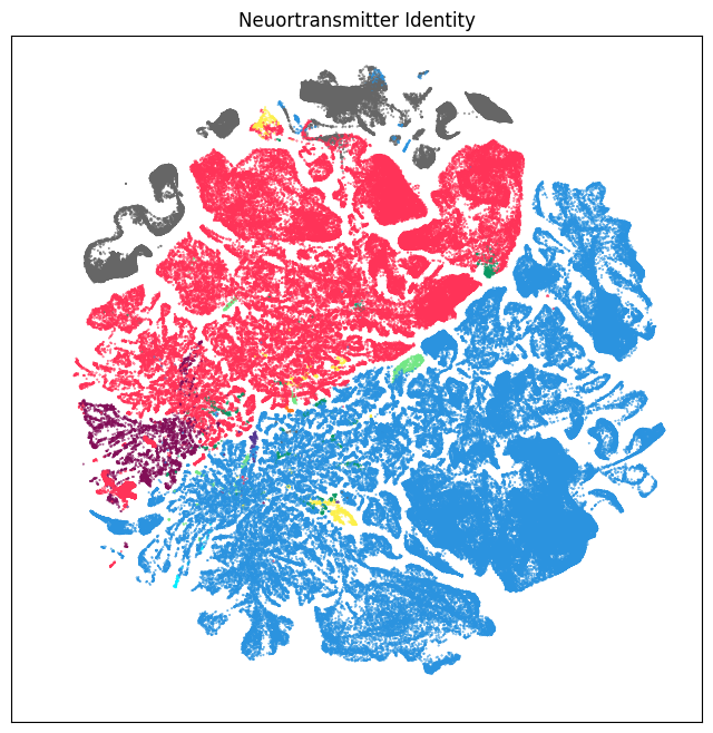
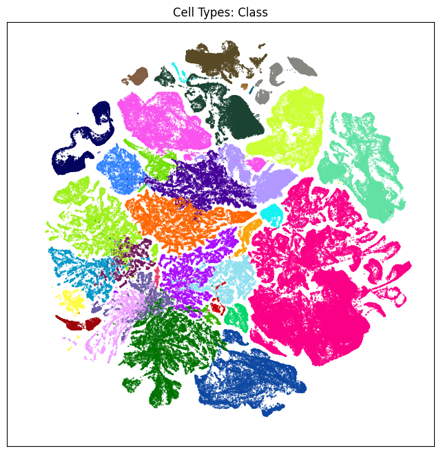
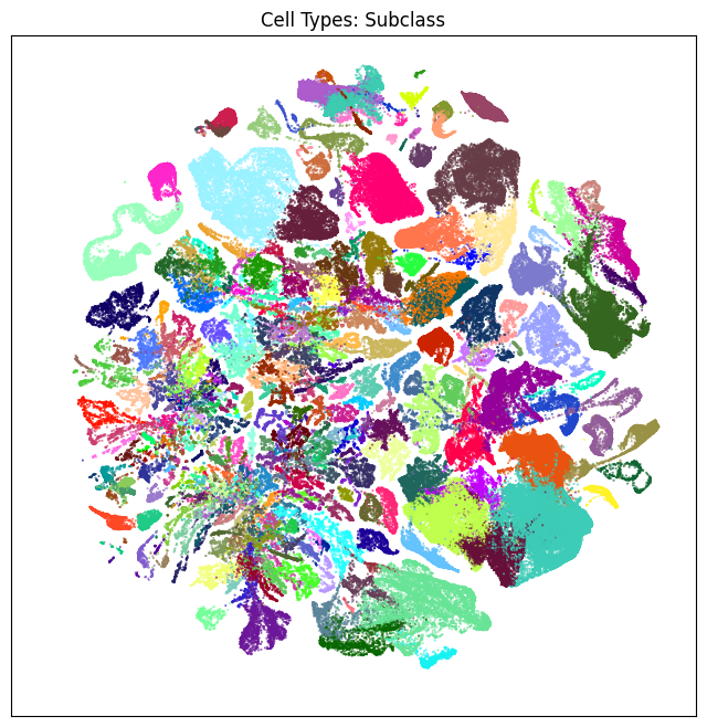
We define a small helper function plot umap to visualize the cells on the UMAP colorized by: dissection region of interest, neurotransmitter identity, cell types division, class and subclass. For ease of demostration, we do a simple subsampling of the cells by a factor of 10 to reduce processing time.
def plot_umap(xx, yy, cc=None, val=None, fig_width=8, fig_height=8, cmap=None):

    fig, ax = plt.subplots()
    fig.set_size_inches(fig_width, fig_height)

    if cmap is not None :
        plt.scatter(xx, yy, s=0.5, c=val, marker='.', cmap=cmap)
    elif cc is not None :
        plt.scatter(xx, yy, s=0.5, color=cc, marker='.')

    ax.axis('equal')
    ax.set_xlim(-18, 27)
    ax.set_ylim(-18, 27)
    ax.set_xticks([])
    ax.set_yticks([])

    return fig, ax
cell_subsampled = cell_extended.loc[::10]
print(len(cell_subsampled))
404298
fig, ax = plot_umap(cell_subsampled['x'], cell_subsampled['y'], cc=cell_subsampled['region_of_interest_color'])
res = ax.set_title("Dissection Region Of Interest")
plt.show()
fig, ax = plot_umap(cell_subsampled['x'], cell_subsampled['y'], cc=cell_subsampled['neurotransmitter_color'])
res = ax.set_title("Neuortransmitter Identity")
plt.show()
fig, ax = plot_umap(cell_subsampled['x'], cell_subsampled['y'], cc=cell_subsampled['class_color'])
res = ax.set_title("Cell Types: Class")
plt.show()
fig, ax = plot_umap(cell_subsampled['x'], cell_subsampled['y'], cc=cell_subsampled['subclass_color'])
res = ax.set_title("Cell Types: Subclass")
plt.show()
Single cell transcriptomes#
Each 10x library was sequenced on the Illumina NovaSeq6000 platform, and sequencing reads were aligned to the mouse reference transcriptome mm10 (GENCODE vM23/Ensembl 98) using the 10x Genomics CellRanger pipeline (version 6.1.1) with default parameters. Each gene is uniquely identifier by an Ensembl ID. It is best practice to gene identifier to for tracking and data interchange as gene symbols are not unique and can change over time
Each row of the gene dataframe has Ensembl gene identifier, a gene symbol and name. 1173 genes have no expression across all the cells in the dataset and can be identified by “no expression” in the comment column.
gene = abc_cache.get_metadata_dataframe(directory='WMB-10X', file_name='gene')
gene.set_index('gene_identifier', inplace=True)
print("Number of genes = ", len(gene))
gene.head(5)
Number of genes = 32285
| gene_symbol | name | mapped_ncbi_identifier | comment | |
|---|---|---|---|---|
| gene_identifier | ||||
| ENSMUSG00000051951 | Xkr4 | X-linked Kx blood group related 4 | NCBIGene:497097 | NaN |
| ENSMUSG00000089699 | Gm1992 | predicted gene 1992 | NaN | NaN |
| ENSMUSG00000102331 | Gm19938 | predicted gene, 19938 | NaN | NaN |
| ENSMUSG00000102343 | Gm37381 | predicted gene, 37381 | NaN | NaN |
| ENSMUSG00000025900 | Rp1 | retinitis pigmentosa 1 (human) | NCBIGene:19888 | NaN |
pred = (gene['comment'] == 'no expression')
filtered = gene[pred]
print("Number of no expression genes", len(filtered))
filtered
Number of no expression genes 1173
| gene_symbol | name | mapped_ncbi_identifier | comment | |
|---|---|---|---|---|
| gene_identifier | ||||
| ENSMUSG00000118272 | Arhgef4 | Rho guanine nucleotide exchange factor (GEF) 4 | NaN | no expression |
| ENSMUSG00000117809 | Asdurf | Asnsd1 upstream reading frame | NCBIGene:110599589 | no expression |
| ENSMUSG00000047383 | AC169382.1 | novel transcript | NaN | no expression |
| ENSMUSG00000097001 | 1700054K02Rik | RIKEN cDNA 1700054K02 gene | NaN | no expression |
| ENSMUSG00000116048 | Sept2 | septin 2 | NaN | no expression |
| ... | ... | ... | ... | ... |
| ENSMUSG00000091585 | AC140365.1 | PRAME family member 8-like | NaN | no expression |
| ENSMUSG00000095523 | AC124606.1 | PRAME family member 8-like | NCBIGene:100038995 | no expression |
| ENSMUSG00000095475 | AC133095.2 | uncharacterized LOC545763 | NCBIGene:545763 | no expression |
| ENSMUSG00000094855 | AC133095.1 | uncharacterized LOC620639 | NCBIGene:620639 | no expression |
| ENSMUSG00000095019 | AC234645.1 | NaN | NaN | no expression |
1173 rows × 4 columns
Gene expression matrices#
The 4 million cell dataset has been divided into 24 expression matrices to make data transfer and download more efficient. Each package is formatted as an annadata h5ad file with minimal metadata. In this next section, we provide example code on how to open one of the expression matrix files and connect with the rich cell level metadata discussed above.
For each subset, there are two h5ad files one storing the raw counts and the other log normalization of it. For this example, we will use the log2 version of the expression matrix.
Below we list the available files in the WMB-10Xv2 directoy and load the WMB-10Xv2-TH data.
abc_cache.list_expression_matrix_files('WMB-10Xv2')
['WMB-10Xv2-CTXsp/log2',
 'WMB-10Xv2-CTXsp/raw',
 'WMB-10Xv2-HPF/log2',
 'WMB-10Xv2-HPF/raw',
 'WMB-10Xv2-HY/log2',
 'WMB-10Xv2-HY/raw',
 'WMB-10Xv2-Isocortex-1/log2',
 'WMB-10Xv2-Isocortex-1/raw',
 'WMB-10Xv2-Isocortex-2/log2',
 'WMB-10Xv2-Isocortex-2/raw',
 'WMB-10Xv2-Isocortex-3/log2',
 'WMB-10Xv2-Isocortex-3/raw',
 'WMB-10Xv2-Isocortex-4/log2',
 'WMB-10Xv2-Isocortex-4/raw',
 'WMB-10Xv2-MB/log2',
 'WMB-10Xv2-MB/raw',
 'WMB-10Xv2-OLF/log2',
 'WMB-10Xv2-OLF/raw',
 'WMB-10Xv2-TH/log2',
 'WMB-10Xv2-TH/raw']
feature_matrix_label = 'WMB-10Xv2-TH'
file = abc_cache.get_file_path(directory='WMB-10Xv2', file_name='WMB-10Xv2-TH/log2')
print(file)
WMB-10Xv2-TH-log2.h5ad: 100%|██████████| 4.04G/4.04G [09:00<00:00, 7.48MMB/s]
/Users/chris.morrison/src/data/abc_atlas/expression_matrices/WMB-10Xv2/20230630/WMB-10Xv2-TH-log2.h5ad
We use the anndata’s read_h5ad function to open the package for the log2 normalization file. The “backed=’r’” makes use of the lazy loading functionality to only load required data. By default, anndata will load the entire expression matrix in memory.
adata = anndata.read_h5ad(file, backed='r')
print(adata)
AnnData object with n_obs × n_vars = 131212 × 32285 backed at '/Users/chris.morrison/src/data/abc_atlas/expression_matrices/WMB-10Xv2/20230630/WMB-10Xv2-TH-log2.h5ad'
    obs: 'cell_barcode', 'library_label', 'anatomical_division_label'
    var: 'gene_symbol'
    uns: 'normalization', 'parent', 'parent_layer', 'parent_rows'
Genes are represented as “variables”. For this data, the var dataframe is indexed by the Ensembl gene identifier with one metadata column gene symbol.
print("Number of genes = ", len(adata.var))
adata.var.index[0:5]
Number of genes = 32285
Index(['ENSMUSG00000051951', 'ENSMUSG00000089699', 'ENSMUSG00000102331',
       'ENSMUSG00000102343', 'ENSMUSG00000025900'],
      dtype='object', name='gene_identifier')
Cells are represented as “observations”. For this data, the obs dataframe is index by cell label with three minimal metadata columns cell barcode, library label and anatomical division label.
print("Number of cells = ", len(adata.obs))
adata.obs.index[0:5]
Number of cells = 131212
Index(['CAGGTGCAGGCTAGCA-040_C01', 'TGCGCAGGTTGCGCAC-045_C01',
       'CGATGTATCTTGCCGT-042_B01', 'GACTAACGTCCTCTTG-040_B01',
       'GATCGTACAACTGCTA-040_B01'],
      dtype='object', name='cell_label')
We can easily connect the cells in the package to the extended cell metadata with simple pandas filtering.
pred = (cell_extended['feature_matrix_label'] == feature_matrix_label)
cell_filtered = cell_extended[pred]
print("Number of cells = ", len(cell_filtered))
Number of cells = 130555
Example use cases#
In this section, we explore two use cases. The first example looks at the expression of nine canonical neurotransmitter transporter genes and the second the expression of gene Tac2.
To support these use cases, we will create a smaller submatrix (all cells and 10 genes) that read it into memory. Note this operation takes around 10 seconds.
ntgenes = ['Slc17a7', 'Slc17a6', 'Slc17a8', 'Slc32a1', 'Slc6a5', 'Slc18a3', 'Slc6a3', 'Slc6a4', 'Slc6a2']
exgenes = ['Tac2']
gnames = ntgenes + exgenes
pred = [x in gnames for x in adata.var.gene_symbol]
gene_filtered = adata.var[pred]
gene_filtered
| gene_symbol | |
|---|---|
| gene_identifier | |
| ENSMUSG00000037771 | Slc32a1 |
| ENSMUSG00000070570 | Slc17a7 |
| ENSMUSG00000039728 | Slc6a5 |
| ENSMUSG00000030500 | Slc17a6 |
| ENSMUSG00000055368 | Slc6a2 |
| ENSMUSG00000019935 | Slc17a8 |
| ENSMUSG00000025400 | Tac2 |
| ENSMUSG00000020838 | Slc6a4 |
| ENSMUSG00000021609 | Slc6a3 |
| ENSMUSG00000100241 | Slc18a3 |
start = time.process_time()
asubset = adata[:, gene_filtered.index].to_memory()
print("time taken: ", time.process_time() - start)
print(asubset)
time taken:  2.795550999999989
AnnData object with n_obs × n_vars = 131212 × 10
    obs: 'cell_barcode', 'library_label', 'anatomical_division_label'
    var: 'gene_symbol'
    uns: 'normalization', 'parent', 'parent_layer', 'parent_rows'
We define two helper functions to (1) create_expression_dataframe: create joined gene expression and cell metadata dataframe based for a set of input genes and (2) aggregate_by_metadata which computes the average expression for each term in a given category.
def create_expression_dataframe(ad, gf) :
    gdata = ad[:, gf.index].to_df()
    gdata.columns = gf.gene_symbol
    joined = cell_filtered.join(gdata)
    return joined
def aggregate_by_metadata(df, gnames, value, sort=False):
    grouped = df.groupby(value)[gnames].mean()
    if sort:
        grouped = grouped.sort_values(by=gnames[0], ascending=False)
    return grouped
Expression of canonical neurotransmitter transporter genes in the thalamus#
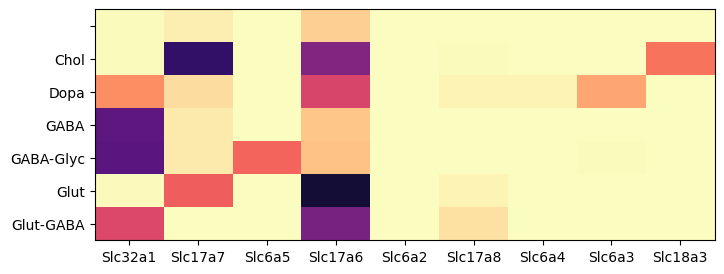
During analysis, clusters were assigned neurotransmitter identities based on the expression of of canonical neurotransmitter transporter genes. In this example, we create a dataframe comprising of cells in the ‘WMB-10Xv2-TH’ package and expression of the 9 solute carrier family genes. We then group the cells by the assigned neurotransmitter class and compute the mean expression for each group. We define a helper function that display a dataframe as a heatmap for visualization.
def plot_heatmap(df, fig_width = 8, fig_height = 4, cmap=plt.cm.magma_r, vmax=None):

    arr = df.to_numpy()

    fig, ax = plt.subplots()
    fig.set_size_inches(fig_width, fig_height)

    res = ax.imshow(arr, cmap=cmap, aspect='auto', vmax=vmax)
    xlabs = df.columns.values
    ylabs = df.index.values

    ax.set_xticks(range(len(xlabs)))
    ax.set_xticklabels(xlabs)

    ax.set_yticks(range(len(ylabs)))
    res = ax.set_yticklabels(ylabs)
Within the thalamus, Slc17a7 is most enriched in cholinergic assigned cells with some expression in glutamatergic types. Genes Slc17a6 is enriched in glutamatergic, Slc32a1 in GABAergic, Slc6a5 in glycinergic, Slc18a3 in cholinergic and Slc6a3 in dopaminergic types, matching the expectation described in the manuscript.
pred = [x in ntgenes for x in asubset.var.gene_symbol]
gf = asubset.var[pred]

ntexp = create_expression_dataframe(asubset, gf)
agg = aggregate_by_metadata(ntexp, gf.gene_symbol, 'neurotransmitter')
plot_heatmap(df=agg, fig_width=8, fig_height=3, vmax=10)
plt.show()
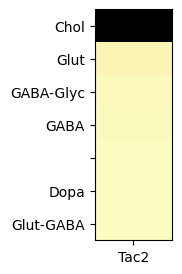
Expression of Tachykinin 2 (Tac2) in the thalamus#
In mice, the tachykinin 2 (Tac2) gene encodes neuropeptide called neurokinin B (NkB). Tac2 is produced by neurons in specific regions of the brain know to be invovled in emotion and social behavior. Based on ISH data from the Allen Mouse Brain Atlas, Tac 2 is sparsely expressed in the mouse isocortex and densely enriched is specific subcortical regions such the medial habenula (MH), the amygdala and hypothalamus.
In this example, we create a dataframe comprising of cells in the ‘WMB-10Xv2-TH’ package and expression values of Tac2 in those cells.
gf = asubset.var[asubset.var.gene_symbol == 'Tac2']
tac2 = create_expression_dataframe(asubset, gf)
Grouping cells by neurotransmitter identites and computing the mean expression in each group, we can observed that Tac2 gene is highly enriched in cholinergic cell types.
agg = aggregate_by_metadata(tac2, gf.gene_symbol, 'neurotransmitter', True).head(10)
plot_heatmap(agg, 1, 3)
plt.show()
/var/folders/kc/7glrmt5n67x16yj_tg86t49c0000gp/T/ipykernel_34072/199257058.py:4: FutureWarning: Series.__getitem__ treating keys as positions is deprecated. In a future version, integer keys will always be treated as labels (consistent with DataFrame behavior). To access a value by position, use `ser.iloc[pos]`
  grouped = grouped.sort_values(by=gnames[0], ascending=False)
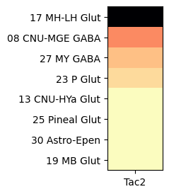
Grouping cells by cell types class, shows that Tac2 is enriched in class “16 MH-LH Glut” with cells restricted to the medial (MH) and lateral (LH) habenula and a mixture of glutamatergic and cholinergic types.
agg = aggregate_by_metadata(tac2, gf.gene_symbol, 'class', True).head(8)
plot_heatmap(agg, 1, 3)
plt.show()
/var/folders/kc/7glrmt5n67x16yj_tg86t49c0000gp/T/ipykernel_34072/199257058.py:4: FutureWarning: Series.__getitem__ treating keys as positions is deprecated. In a future version, integer keys will always be treated as labels (consistent with DataFrame behavior). To access a value by position, use `ser.iloc[pos]`
  grouped = grouped.sort_values(by=gnames[0], ascending=False)
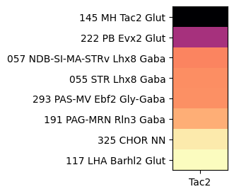
At the next level, grouping by subclass, shows Tac2 is enriched in sublcass “145 MH Tac2 Glut” with further specificity to the medial habenula and with Tac2 itself as a marker for the subclass.
agg = aggregate_by_metadata(tac2, gf.gene_symbol, 'subclass', True).head(8)
plot_heatmap(agg, 1, 3)
plt.show()
/var/folders/kc/7glrmt5n67x16yj_tg86t49c0000gp/T/ipykernel_34072/199257058.py:4: FutureWarning: Series.__getitem__ treating keys as positions is deprecated. In a future version, integer keys will always be treated as labels (consistent with DataFrame behavior). To access a value by position, use `ser.iloc[pos]`
  grouped = grouped.sort_values(by=gnames[0], ascending=False)
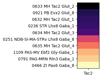
Next level down, gene Tac2 is enriched in several children supertypes of “145 MH Tac2 Glut”
agg = aggregate_by_metadata(tac2, gf.gene_symbol, 'supertype', True).head(10)
plot_heatmap(agg, 1, 3)
plt.show()
/var/folders/kc/7glrmt5n67x16yj_tg86t49c0000gp/T/ipykernel_34072/199257058.py:4: FutureWarning: Series.__getitem__ treating keys as positions is deprecated. In a future version, integer keys will always be treated as labels (consistent with DataFrame behavior). To access a value by position, use `ser.iloc[pos]`
  grouped = grouped.sort_values(by=gnames[0], ascending=False)
Close h5ad file and clean up
adata.file.close()
del adata