MERFISH CCF mapped coordinates#
Registration to the Allen CCFv3 was performed at 10 micron in-plane resolution. For each section, an anatomical label reference was created using class/subclass level cell type assignments which are then used to match to corresponding CCF parcellations. The midline was manually determined for each section to rotate the section upright and center in in the middle (section coordinates). This set of rectified images were stacked in sequential order to create an inital configuration for registration.
The ANTS registration framework was use to establish a 2.5D deformable spatial mapping between the MERFISH data and CCF coordinates via three major steps: (1) A 3D global affine (12 dof) mapping was performed to align the CCF into the MERFISH space (resampled CCF); (2) 2D affine (6 dof) registration of each MERFISH section to match the target resampled CCF section and finally, (3) a 2D multi-scale, symmetric diffeomorphic registration of each section (reconstructed coordinates) to finer level match to the target CCF section. Global and section-wise mappings from each of these registration steps were preserved and concatenated (with appropriate inversions) to allow point-to-point mapping between the original MERFISH coordinate space and the CCF space. See Yao et al for further details.
The purpose of this notebook is to provide an overview of how the mapped coordinate information is represented through example use cases.
You need to be connected to the internet to run this notebook and have run through the getting started notebook.
import pandas as pd
import numpy as np
import matplotlib.pyplot as plt
import SimpleITK as sitk
from pathlib import Path

from abc_atlas_access.abc_atlas_cache.abc_project_cache import AbcProjectCache
We will interact with the data using the AbcProjectCache. This cache object tracks which data has been downloaded and serves the path to the requsted data on disk. For metadata, the cache can also directly serve a up a Pandas Dataframe. See the getting_started notebook for more details on using the cache including installing it if it has not already been.
Change the download_base variable to where you have downloaded the data in your system.
download_base = Path('../../data/abc_atlas')
abc_cache = AbcProjectCache.from_cache_dir(download_base)

abc_cache.current_manifest
'releases/20250531/manifest.json'
Read in section, reconstructed and CCF coordinates for all cells#
Read in the expanded cell metadata table we created in part 1 of the MERFISH tutorial. To keep track of the three type of coordinates we will rename the section coordinates (x,y,z) in the dataframe to (x_section, y_section, z_section)
cell = abc_cache.get_metadata_dataframe(directory='MERFISH-C57BL6J-638850', file_name='cell_metadata_with_cluster_annotation')
cell.rename(columns={'x': 'x_section',
                     'y': 'y_section',
                     'z': 'z_section'},
            inplace=True)
cell.set_index('cell_label', inplace=True)
cell.head(5)
| brain_section_label | cluster_alias | average_correlation_score | feature_matrix_label | donor_label | donor_genotype | donor_sex | x_section | y_section | z_section | neurotransmitter | class | subclass | supertype | cluster | neurotransmitter_color | class_color | subclass_color | supertype_color | cluster_color | |
|---|---|---|---|---|---|---|---|---|---|---|---|---|---|---|---|---|---|---|---|---|
| cell_label | ||||||||||||||||||||
| 1019171907102340387-1 | C57BL6J-638850.37 | 1408 | 0.596276 | C57BL6J-638850 | C57BL6J-638850 | wt/wt | M | 7.226245 | 4.148963 | 6.6 | NaN | 04 DG-IMN Glut | 038 DG-PIR Ex IMN | 0141 DG-PIR Ex IMN_2 | 0515 DG-PIR Ex IMN_2 | #666666 | #16f2f2 | #3D53CC | #CC7A3D | #73FFBF |
| 1104095349101460194-1 | C57BL6J-638850.26 | 4218 | 0.641180 | C57BL6J-638850 | C57BL6J-638850 | wt/wt | M | 5.064889 | 7.309543 | 4.2 | Glut | 23 P Glut | 235 PG-TRN-LRN Fat2 Glut | 0953 PG-TRN-LRN Fat2 Glut_1 | 4199 PG-TRN-LRN Fat2 Glut_1 | #2B93DF | #6b5ca5 | #9B7ACC | #990041 | #663D63 |
| 1017092617101450577 | C57BL6J-638850.25 | 4218 | 0.763531 | C57BL6J-638850 | C57BL6J-638850 | wt/wt | M | 5.792921 | 8.189973 | 4.0 | Glut | 23 P Glut | 235 PG-TRN-LRN Fat2 Glut | 0953 PG-TRN-LRN Fat2 Glut_1 | 4199 PG-TRN-LRN Fat2 Glut_1 | #2B93DF | #6b5ca5 | #9B7ACC | #990041 | #663D63 |
| 1018093344101130233 | C57BL6J-638850.13 | 4218 | 0.558073 | C57BL6J-638850 | C57BL6J-638850 | wt/wt | M | 3.195950 | 5.868655 | 2.4 | Glut | 23 P Glut | 235 PG-TRN-LRN Fat2 Glut | 0953 PG-TRN-LRN Fat2 Glut_1 | 4199 PG-TRN-LRN Fat2 Glut_1 | #2B93DF | #6b5ca5 | #9B7ACC | #990041 | #663D63 |
| 1019171912201610094 | C57BL6J-638850.27 | 4218 | 0.591009 | C57BL6J-638850 | C57BL6J-638850 | wt/wt | M | 5.635732 | 7.995842 | 4.4 | Glut | 23 P Glut | 235 PG-TRN-LRN Fat2 Glut | 0953 PG-TRN-LRN Fat2 Glut_1 | 4199 PG-TRN-LRN Fat2 Glut_1 | #2B93DF | #6b5ca5 | #9B7ACC | #990041 | #663D63 |
Next we read in the reconstructed coordinates and mapped parcellation from the metadata directory and join it to the cell dataframe
reconstructed_coords = abc_cache.get_metadata_dataframe(
    directory='MERFISH-C57BL6J-638850-CCF',
    file_name='reconstructed_coordinates',
    dtype={"cell_label": str}
)
reconstructed_coords.rename(columns={'x': 'x_reconstructed',
                                     'y': 'y_reconstructed',
                                     'z': 'z_reconstructed'},
                            inplace=True)
reconstructed_coords.set_index('cell_label', inplace=True)
reconstructed_coords.head(5)
| x_reconstructed | y_reconstructed | z_reconstructed | parcellation_index | |
|---|---|---|---|---|
| cell_label | ||||
| 1019171911101460569 | 7.143894 | 7.890964 | 0.8 | 945 |
| 1019171911101550321 | 4.188673 | 7.962972 | 0.8 | 945 |
| 1019171911100841066 | 6.859447 | 5.908534 | 0.8 | 893 |
| 1019171911101400425 | 3.952014 | 7.564086 | 0.8 | 842 |
| 1019171911101380264 | 2.803546 | 7.221688 | 0.8 | 0 |
cell_joined = cell.join(reconstructed_coords, how='inner')
cell_joined.head(5)
| brain_section_label | cluster_alias | average_correlation_score | feature_matrix_label | donor_label | donor_genotype | donor_sex | x_section | y_section | z_section | ... | cluster | neurotransmitter_color | class_color | subclass_color | supertype_color | cluster_color | x_reconstructed | y_reconstructed | z_reconstructed | parcellation_index | |
|---|---|---|---|---|---|---|---|---|---|---|---|---|---|---|---|---|---|---|---|---|---|
| cell_label | |||||||||||||||||||||
| 1019171907102340387-1 | C57BL6J-638850.37 | 1408 | 0.596276 | C57BL6J-638850 | C57BL6J-638850 | wt/wt | M | 7.226245 | 4.148963 | 6.6 | ... | 0515 DG-PIR Ex IMN_2 | #666666 | #16f2f2 | #3D53CC | #CC7A3D | #73FFBF | 7.255606 | 4.007680 | 6.6 | 1160 |
| 1104095349101460194-1 | C57BL6J-638850.26 | 4218 | 0.641180 | C57BL6J-638850 | C57BL6J-638850 | wt/wt | M | 5.064889 | 7.309543 | 4.2 | ... | 4199 PG-TRN-LRN Fat2 Glut_1 | #2B93DF | #6b5ca5 | #9B7ACC | #990041 | #663D63 | 5.036436 | 7.264429 | 4.2 | 564 |
| 1017092617101450577 | C57BL6J-638850.25 | 4218 | 0.763531 | C57BL6J-638850 | C57BL6J-638850 | wt/wt | M | 5.792921 | 8.189973 | 4.0 | ... | 4199 PG-TRN-LRN Fat2 Glut_1 | #2B93DF | #6b5ca5 | #9B7ACC | #990041 | #663D63 | 5.784270 | 8.007646 | 4.0 | 761 |
| 1018093344101130233 | C57BL6J-638850.13 | 4218 | 0.558073 | C57BL6J-638850 | C57BL6J-638850 | wt/wt | M | 3.195950 | 5.868655 | 2.4 | ... | 4199 PG-TRN-LRN Fat2 Glut_1 | #2B93DF | #6b5ca5 | #9B7ACC | #990041 | #663D63 | 3.161528 | 5.719814 | 2.4 | 718 |
| 1019171912201610094 | C57BL6J-638850.27 | 4218 | 0.591009 | C57BL6J-638850 | C57BL6J-638850 | wt/wt | M | 5.635732 | 7.995842 | 4.4 | ... | 4199 PG-TRN-LRN Fat2 Glut_1 | #2B93DF | #6b5ca5 | #9B7ACC | #990041 | #663D63 | 5.618763 | 7.847877 | 4.4 | 761 |
5 rows × 24 columns
We repeat the process for the cell CCF coordinates
ccf_coords = abc_cache.get_metadata_dataframe(
    directory='MERFISH-C57BL6J-638850-CCF',
    file_name='ccf_coordinates',
    dtype={"cell_label": str}
)
ccf_coords.rename(columns={'x': 'x_ccf',
                           'y': 'y_ccf',
                           'z': 'z_ccf'},
                  inplace=True)
ccf_coords.drop(['parcellation_index'], axis=1, inplace=True)
ccf_coords.set_index('cell_label', inplace=True)
ccf_coords.head(5)
| x_ccf | y_ccf | z_ccf | |
|---|---|---|---|
| cell_label | |||
| 1019171911101460569 | 12.282330 | 6.987808 | 7.385773 |
| 1019171911101550321 | 12.192214 | 7.002155 | 4.366855 |
| 1019171911100841066 | 12.500341 | 4.750392 | 7.074634 |
| 1019171911101400425 | 12.231647 | 6.544816 | 4.128568 |
| 1019171911101380264 | 12.238502 | 6.135836 | 2.948194 |
cell_joined = cell_joined.join(ccf_coords, how='inner')
cell_joined.head(5)
| brain_section_label | cluster_alias | average_correlation_score | feature_matrix_label | donor_label | donor_genotype | donor_sex | x_section | y_section | z_section | ... | subclass_color | supertype_color | cluster_color | x_reconstructed | y_reconstructed | z_reconstructed | parcellation_index | x_ccf | y_ccf | z_ccf | |
|---|---|---|---|---|---|---|---|---|---|---|---|---|---|---|---|---|---|---|---|---|---|
| cell_label | |||||||||||||||||||||
| 1019171907102340387-1 | C57BL6J-638850.37 | 1408 | 0.596276 | C57BL6J-638850 | C57BL6J-638850 | wt/wt | M | 7.226245 | 4.148963 | 6.6 | ... | #3D53CC | #CC7A3D | #73FFBF | 7.255606 | 4.007680 | 6.6 | 1160 | 7.495417 | 2.445872 | 7.455066 |
| 1104095349101460194-1 | C57BL6J-638850.26 | 4218 | 0.641180 | C57BL6J-638850 | C57BL6J-638850 | wt/wt | M | 5.064889 | 7.309543 | 4.2 | ... | #9B7ACC | #990041 | #663D63 | 5.036436 | 7.264429 | 4.2 | 564 | 9.227966 | 6.133693 | 5.225024 |
| 1017092617101450577 | C57BL6J-638850.25 | 4218 | 0.763531 | C57BL6J-638850 | C57BL6J-638850 | wt/wt | M | 5.792921 | 8.189973 | 4.0 | ... | #9B7ACC | #990041 | #663D63 | 5.784270 | 8.007646 | 4.0 | 761 | 9.344912 | 6.989939 | 6.002664 |
| 1018093344101130233 | C57BL6J-638850.13 | 4218 | 0.558073 | C57BL6J-638850 | C57BL6J-638850 | wt/wt | M | 3.195950 | 5.868655 | 2.4 | ... | #9B7ACC | #990041 | #663D63 | 3.161528 | 5.719814 | 2.4 | 718 | 10.977068 | 4.398568 | 3.305223 |
| 1019171912201610094 | C57BL6J-638850.27 | 4218 | 0.591009 | C57BL6J-638850 | C57BL6J-638850 | wt/wt | M | 5.635732 | 7.995842 | 4.4 | ... | #9B7ACC | #990041 | #663D63 | 5.618763 | 7.847877 | 4.4 | 761 | 8.997138 | 6.798329 | 5.827197 |
5 rows × 27 columns
Visualize cells in section, reconstruced and CCF coordinates#
We define a helper function to visualize cells in a section colorized by either cluster or annotation term and optionally with a boundary overlay
def plot_section(xx=None, yy=None, cc=None, val=None, pcmap=None,
                 overlay=None, extent=None, bcmap=plt.cm.Greys_r, alpha=1.0,
                 fig_width = 6, fig_height = 6):

    fig, ax = plt.subplots()
    fig.set_size_inches(fig_width, fig_height)

    if xx is not None and yy is not None and pcmap is not None:
        plt.scatter(xx, yy, s=0.5, c=val, marker='.', cmap=pcmap)
    elif xx is not None and yy is not None and cc is not None:
        plt.scatter(xx, yy, s=0.5, color=cc, marker='.', zorder=1)

    if overlay is not None and extent is not None and bcmap is not None:
        plt.imshow(overlay, cmap=bcmap, extent=extent, alpha=alpha, zorder=2)

    ax.set_ylim(11, 0)
    ax.set_xlim(0, 11)
    ax.axis('equal')
    ax.set_xticks([])
    ax.set_yticks([])

    return fig, ax
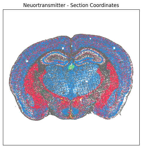
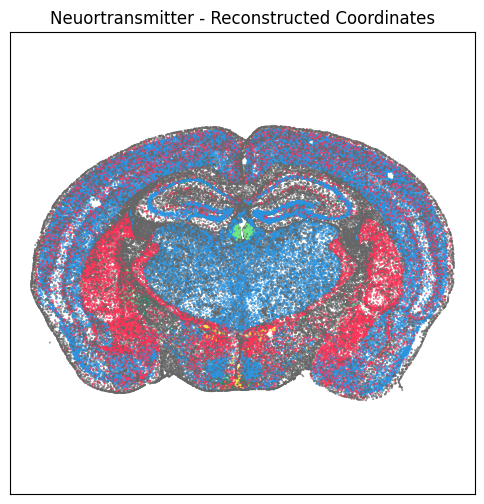
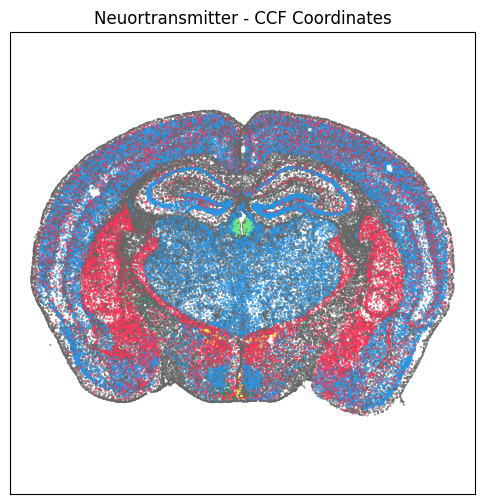
For example section “C57BL6J-638850.40”, we plot cells by section, reconstructed and ccf coordinates colorized by neurotransmitter type assignment. Note that cells from a single brain section remains together at the same z (posterior-to-anterior) value in section and reconstructed coordinates. Since the brain sections are at an angle compared to the CCF, the cells are spread across multiple x (anterior-to-posterior) CCF coordinates.
brain_section = 'C57BL6J-638850.40'
pred = (cell_joined['brain_section_label'] == brain_section)
section = cell_joined[pred]
print(len(section))
104572
print("z_section values:", np.unique(section['z_section']))
print("z_reconstructed values:", np.unique(section['z_reconstructed']))
print("x_ccf values:", np.unique(section['x_ccf']))
z_section values: [7.2]
z_reconstructed values: [7.2]
x_ccf values: [6.32598314 6.32656693 6.3266852  ... 7.16574148 7.16579943 7.16598123]
fig, ax = plot_section(xx=section['x_section'],
                       yy=section['y_section'],
                       cc=section['neurotransmitter_color'])
res = ax.set_title("Neuortransmitter - Section Coordinates")
plt.show()
fig, ax = plot_section(xx=section['x_reconstructed'],
                       yy=section['y_reconstructed'],
                       cc=section['neurotransmitter_color'])
res = ax.set_title("Neuortransmitter - Reconstructed Coordinates")
plt.show()
fig, ax = plot_section(xx=section['z_ccf'],
                       yy=section['y_ccf'],
                       cc=section['neurotransmitter_color'])
res = ax.set_title("Neuortransmitter - CCF Coordinates")
plt.show()
Associate mapped parcellation and parcellation terms to the MERFISH data#
Read in the pivoted parcellation annotation information we created in the Allen CCFv3 tutorial and join with the cell metadata dataframe.
parcellation_annotation = abc_cache.get_metadata_dataframe(directory='Allen-CCF-2020',
                                                           file_name='parcellation_to_parcellation_term_membership_acronym')
parcellation_annotation.set_index('parcellation_index', inplace=True)
parcellation_annotation.columns = ['parcellation_%s'% x for x in  parcellation_annotation.columns]
parcellation_annotation.head(5)
| parcellation_organ | parcellation_category | parcellation_division | parcellation_structure | parcellation_substructure | |
|---|---|---|---|---|---|
| parcellation_index | |||||
| 0 | unassigned | unassigned | unassigned | unassigned | unassigned |
| 1 | brain | grey | HY | TMv | TMv |
| 2 | brain | grey | Isocortex | SSp-m | SSp-m6b |
| 5 | brain | fiber tracts | lfbs | cst | int |
| 6 | brain | grey | P | PSV | PSV |
parcellation_color = abc_cache.get_metadata_dataframe(directory='Allen-CCF-2020',
                                                      file_name='parcellation_to_parcellation_term_membership_color')
parcellation_color.set_index('parcellation_index', inplace=True)
parcellation_color.columns = ['parcellation_%s'% x for x in  parcellation_color.columns]
parcellation_color.head(5)
| parcellation_organ_color | parcellation_category_color | parcellation_division_color | parcellation_structure_color | parcellation_substructure_color | |
|---|---|---|---|---|---|
| parcellation_index | |||||
| 0 | #000000 | #000000 | #000000 | #000000 | #000000 |
| 1 | #FFFFFF | #BFDAE3 | #E64438 | #FF4C3E | #FF4C3E |
| 2 | #FFFFFF | #BFDAE3 | #70FF71 | #188064 | #188064 |
| 5 | #FFFFFF | #CCCCCC | #CCCCCC | #CCCCCC | #CCCCCC |
| 6 | #FFFFFF | #BFDAE3 | #FF9B88 | #FFAE6F | #FFAE6F |
cell_joined = cell_joined.join(parcellation_annotation, on='parcellation_index')
cell_joined = cell_joined.join(parcellation_color, on='parcellation_index')
cell_joined.head(5)
| brain_section_label | cluster_alias | average_correlation_score | feature_matrix_label | donor_label | donor_genotype | donor_sex | x_section | y_section | z_section | ... | parcellation_organ | parcellation_category | parcellation_division | parcellation_structure | parcellation_substructure | parcellation_organ_color | parcellation_category_color | parcellation_division_color | parcellation_structure_color | parcellation_substructure_color | |
|---|---|---|---|---|---|---|---|---|---|---|---|---|---|---|---|---|---|---|---|---|---|
| cell_label | |||||||||||||||||||||
| 1019171907102340387-1 | C57BL6J-638850.37 | 1408 | 0.596276 | C57BL6J-638850 | C57BL6J-638850 | wt/wt | M | 7.226245 | 4.148963 | 6.6 | ... | brain | grey | HPF | DG | DG-po | #FFFFFF | #BFDAE3 | #7ED04B | #7ED04B | #7ED04B |
| 1104095349101460194-1 | C57BL6J-638850.26 | 4218 | 0.641180 | C57BL6J-638850 | C57BL6J-638850 | wt/wt | M | 5.064889 | 7.309543 | 4.2 | ... | brain | grey | P | TRN | TRN | #FFFFFF | #BFDAE3 | #FF9B88 | #FFBA86 | #FFBA86 |
| 1017092617101450577 | C57BL6J-638850.25 | 4218 | 0.763531 | C57BL6J-638850 | C57BL6J-638850 | wt/wt | M | 5.792921 | 8.189973 | 4.0 | ... | brain | grey | P | P-unassigned | P-unassigned | #FFFFFF | #BFDAE3 | #FF9B88 | #FF9B88 | #FF9B88 |
| 1018093344101130233 | C57BL6J-638850.13 | 4218 | 0.558073 | C57BL6J-638850 | C57BL6J-638850 | wt/wt | M | 3.195950 | 5.868655 | 2.4 | ... | brain | fiber tracts | cbf | arb | arb | #FFFFFF | #CCCCCC | #CCCCCC | #CCCCCC | #CCCCCC |
| 1019171912201610094 | C57BL6J-638850.27 | 4218 | 0.591009 | C57BL6J-638850 | C57BL6J-638850 | wt/wt | M | 5.635732 | 7.995842 | 4.4 | ... | brain | grey | P | P-unassigned | P-unassigned | #FFFFFF | #BFDAE3 | #FF9B88 | #FF9B88 | #FF9B88 |
5 rows × 37 columns
The joined DataFrame cell_joined created above is available from the cache as the file cell_metadata_with_parcellation_annotation.
Visualize cell parcellation assignment at different anatomical levels#
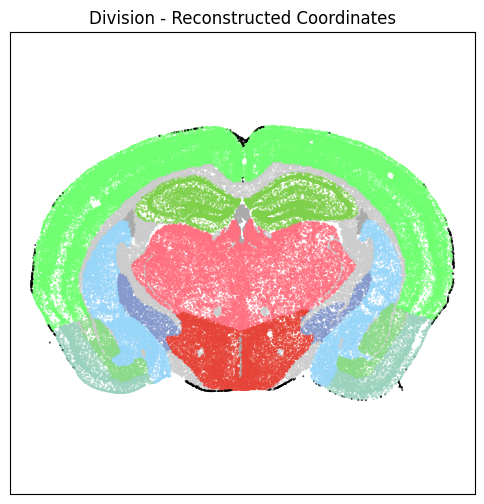
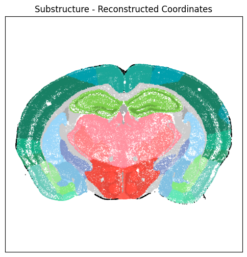
For example section “C57BL6J-638850.40”, we plot cells reconstructed coordinates colorized by parcellation assignment at the division and structure anatomical levels
pred = (cell_joined['brain_section_label'] == brain_section)
section = cell_joined[pred]
print(len(section))
104572
fig, ax = plot_section(xx=section['x_reconstructed'],
                       yy=section['y_reconstructed'],
                       cc=section['parcellation_division_color'])
res = ax.set_title("Division - Reconstructed Coordinates")
plt.show()
fig, ax = plot_section(xx=section['x_reconstructed'],
                       yy=section['y_reconstructed'],
                       cc=section['parcellation_structure_color'])
res = ax.set_title("Structure - Reconstructed Coordinates")
plt.show()

fig, ax = plot_section(xx=section['x_reconstructed'],
                       yy=section['y_reconstructed'],
                       cc=section['parcellation_substructure_color'])
res = ax.set_title("Substructure - Reconstructed Coordinates")
plt.show()
Aggregate cells by parcellation assignment at different anatomical levels#
Define a helper function to count the number of cells for each term and apply it to the division and structure anatomical levels
def parcellation_cell_count (df,level) :
    cell_count = df.groupby(level)[['cluster_alias']].count()
    cell_count.columns = ['number_of_cells']
    cell_count.sort_values('number_of_cells', ascending=False, inplace=True)
    return cell_count
cell_count = parcellation_cell_count(cell_joined, 'parcellation_division')
cell_count.head(10)
| number_of_cells | |
|---|---|
| parcellation_division | |
| Isocortex | 935742 |
| STR | 401346 |
| CB | 383127 |
| HPF | 304642 |
| MB | 281852 |
| OLF | 274354 |
| MY | 147562 |
| P | 136569 |
| TH | 133805 |
| HY | 132902 |
cell_count = parcellation_cell_count(section, 'parcellation_structure')
cell_count.head(10)
| number_of_cells | |
|---|---|
| parcellation_structure | |
| SSp-bfd | 8865 |
| SSs | 7210 |
| CP | 4715 |
| DG | 4491 |
| VISa | 4462 |
| CA1 | 3705 |
| PIR | 3119 |
| cst | 3000 |
| cc | 2858 |
| RSPv | 2853 |
We can filtered cells to specific subclasses and types and count within the filtered set
pred = (cell_joined['subclass'] == '145 MH Tac2 Glut')
filtered = cell_joined[pred]
print("number of cells:", len(filtered))
cell_count = parcellation_cell_count(filtered, 'parcellation_structure')
cell_count.head(10)
number of cells: 4696
| number_of_cells | |
|---|---|
| parcellation_structure | |
| MH | 4404 |
| V3-unassigned | 132 |
| mfsbshy | 73 |
| brain-unassigned | 46 |
| chpl | 21 |
| LH | 12 |
| DG | 3 |
| TH-unassigned | 2 |
| LP | 1 |
| MD | 1 |
pred = (cell_joined['subclass'] == '146 LH Pou4f1 Sox1 Glut')
filtered = cell_joined[pred]
print("number of cells:", len(filtered))
cell_count = parcellation_cell_count(filtered, 'parcellation_structure')
cell_count.head(10)
number of cells: 1067
| number_of_cells | |
|---|---|
| parcellation_structure | |
| LH | 851 |
| mfsbshy | 109 |
| MH | 59 |
| PAG | 10 |
| TH-unassigned | 10 |
| brain-unassigned | 7 |
| PF | 6 |
| DG | 5 |
| MD | 4 |
| SPA | 2 |
pred = (cell_joined['subclass'] == '147 AD Serpinb7 Glut')
filtered = cell_joined[pred]
print("number of cells:", len(filtered))
cell_count = parcellation_cell_count(filtered, 'parcellation_structure')
cell_count.head(10)
number of cells: 1190
| number_of_cells | |
|---|---|
| parcellation_structure | |
| AD | 1036 |
| mfsbshy | 84 |
| brain-unassigned | 35 |
| DG | 22 |
| LD | 4 |
| AM | 3 |
| TH-unassigned | 3 |
| mfbc | 3 |
pred = (cell_joined['subclass'] == '007 L2/3 IT CTX Glut')
filtered = cell_joined[pred]
print("number of cells:", len(filtered))
cell_count = parcellation_cell_count(filtered, 'parcellation_substructure')
cell_count.head(10)
number of cells: 121784
| number_of_cells | |
|---|---|
| parcellation_substructure | |
| MOs2/3 | 12762 |
| MOp2/3 | 10586 |
| VISp2/3 | 9250 |
| SSs2/3 | 7149 |
| SSp-m2/3 | 5203 |
| SSp-bfd2/3 | 5032 |
| TEa2/3 | 4396 |
| SSp-ul2/3 | 3337 |
| RSPagl2/3 | 3142 |
| ACAv2/3 | 3085 |
Resampled CCF template and parcellations#
The anatomical template, parcellation and boundary volume in resample CCF coordinates are also available for download for visualization and analysis
abc_cache.list_image_volume_files('MERFISH-C57BL6J-638850-CCF')
['resampled_annotation',
 'resampled_annotation_boundary',
 'resampled_average_template']
print("reading resampled_average_template")
file = abc_cache.get_file_path(directory='MERFISH-C57BL6J-638850-CCF',
                               file_name='resampled_average_template')
average_template_image = sitk.ReadImage(file)
average_template_array = sitk.GetArrayViewFromImage(average_template_image)

print("reading resampled_annotation")
file = abc_cache.get_file_path(directory='MERFISH-C57BL6J-638850-CCF',
                               file_name='resampled_annotation')
annotation_image = sitk.ReadImage(file)
annotation_array = sitk.GetArrayViewFromImage(annotation_image)

print("reading resampled_annotation_boundary")
file = abc_cache.get_file_path(directory='MERFISH-C57BL6J-638850-CCF',
                               file_name='resampled_annotation_boundary')
annotation_boundary_image = sitk.ReadImage(file)
annotation_boundary_array = sitk.GetArrayViewFromImage(annotation_boundary_image)
reading resampled_average_template
reading resampled_annotation
reading resampled_annotation_boundary
# Function to print out image information
def image_info(img):
    print('size: ' + str(img.GetSize()) + ' voxels')
    print('spacing: ' + str(img.GetSpacing()) + ' mm' )
    print('direction: ' + str(img.GetDirection()) )
    print('origin: ' + str(img.GetOrigin()))
image_info(average_template_image)
size: (1100, 1100, 76) voxels
spacing: (0.009999999776482582, 0.009999999776482582, 0.20000000298023224) mm
direction: (-1.0, 0.0, 0.0, 0.0, -0.0, -1.0, 0.0, -1.0, 0.0)
origin: (5.476531505584717, 8.600000381469727, 6.435669422149658)
To enable the overlay of image section with cell coordinates we need to compute the extent the image in mm coordinates
size = average_template_image.GetSize()
spacing = average_template_image.GetSpacing()
extent = (-0.5 * spacing[0], (size[0]-0.5) * spacing[0], (size[1]-0.5) * spacing[1], -0.5 * spacing[1])
Visualize cells with parcellation boundary overlay#
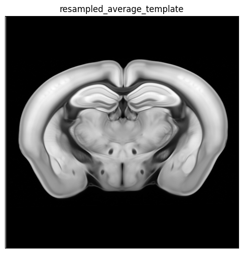
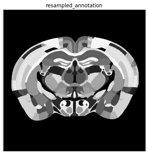
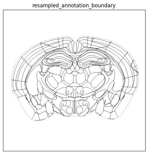
For example section “C57BL6J-638850.40”, we first compute the corresponding z section in the resampled image volume and visualize the resampled average template, annotation and parcellation for that section
zindex = int(section.iloc[0]['z_reconstructed'] / 0.2)
zindex
36
template_slice = average_template_array[zindex, :, :]
fig, ax = plot_section(overlay=template_slice, extent=extent)
res = ax.set_title('resampled_average_template')
plt.show()
annotation_slice = annotation_array[zindex, :, :]
fig, ax = plot_section(overlay=annotation_slice, extent=extent)
res = ax.set_title('resampled_annotation')
plt.show()
boundary_slice = annotation_boundary_array[zindex, :, :]
fig, ax = plot_section(overlay=boundary_slice, bcmap=plt.cm.Greys, extent=extent)
res = ax.set_title('resampled_annotation_boundary')
plt.show()
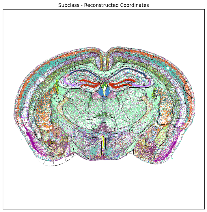
Using the help function, we can overlay the parcellation boundary overlay on top of the cells colorized by subclass
fig, ax = plot_section(section['x_reconstructed'],
                       section['y_reconstructed'],
                       cc=section['subclass_color'],
                       overlay=boundary_slice,
                       extent=extent,
                       bcmap=plt.cm.Greys,
                       alpha = 1.0*(boundary_slice>0),
                       fig_width = 9,
                       fig_height = 9 )
res = ax.set_title("Subclass - Reconstructed Coordinates")
plt.show()