ASAP Human Postmortem-Derived Brain Sequencing Collection (PMDBS): Data Overview

Aligning Science Across Parkinson’s (ASAP), The Michael J. Fox Foundation for Parkinson’s Research (MJFF), and the Allen Institute for Brain Science (AIBS) are teaming up to further the mission of the ASAP Collaborative Research Network (CRN) program, to accelerate discoveries in the Parkinson’s disease (PD) and neurodegenerative disease research communities. Together we will annotate, enhance and add knowledge to the growing data catalog in the ASAP CRN Cloud through integration of cell type taxonomies using the Allen Institute’s MapMyCells tool and visualization through the Allen Brain Cell (ABC) Atlas web application. This integration of data and knowledge will allow users to visualize and explore the changes in gene expression of specific, highly resolved brain cell types in the context of a large PD cohort of donors.

This initial collaboration focuses on the Human Postmortem-derived Brain Sequencing Collection (PMDBS), a harmonized repository comprised of single nucleus and PolyA RNA-seq data contributed by five ASAP CRN teams (Hafler, Lee, Jakobsson, Scherzer, Hardy). Sequencing data were uniformly aligned to the GRCh38.p13 reference genome (Gencode V32), quality control was performed and low-quality cells were filtered out. A set of highly variable genes were identified and the scVI workflow resulted in an integrated latent variable representation, 2D UMAP coordinates and a set of 30 clusters. Currently, the repository spans roughly 3 millions cells obtained from 9 brain regions and 211 donors with various pathologies (including healthy control). For more details on this dataset and to access the raw data used in its preparation, please visit the ASAP CRN Cloud webpage.

In this notebook we assemble the metadata associated with individual cells derived from donor, sample and data integration process information.

You need to be connected to the internet to run this notebook and should have run through the getting started notebook.

import anndata
import matplotlib.pyplot as plt
import numpy as np
import pandas as pd
from pathlib import Path

from abc_atlas_access.abc_atlas_cache.abc_project_cache import AbcProjectCache

We will interact with the data using the AbcProjectCache. This cache object tracks which data has been downloaded and serves the path to the requested data on disk. For metadata, the cache can also directly serve up a Pandas DataFrame. See the getting started notebook notebook for more details on using the cache including installing it if it has not already been.

Change the download_base variable to where you have downloaded the data in your system.

download_base = Path('../../data/abc_atlas')
abc_cache = AbcProjectCache.from_cache_dir(download_base)

abc_cache.current_manifest

'releases/20250331/manifest.json'

Data Overview

ASAP Data

We simplify the ASAP-PMDB metadata into a single cell_metadata.csv file and companion tables describing the donor (including sex, age, race, disease state etc.), sample (including data processing metadata, team information, and region of interest from which the sample was dissected from), and value_sets.csv which provides a mapping from unique terms to their plotting color and term order.

We’ll first load the cell metadata. This provides the UMAP x, y coordinates and clusters provided by ASAP. Refer to the collection documentation for description of the data processing and source datasets.

cell_metadata = abc_cache.get_metadata_dataframe(
    directory='ASAP-PMDBS-10X',
    file_name='cell_metadata'
).set_index('cell_label')
print("Number of cells = ", len(cell_metadata))
cell_metadata.head()

cell_metadata.csv: 100%|███████████████████████████████████████████████████████████████████████| 555M/555M [01:43<00:00, 5.37MMB/s]

Number of cells =  2796736

	cell_barcode	sample_label	x	y	cluster_label	cluster_label_order	cluster_label_color	dataset_label	feature_matrix_label	abc_sample_id
cell_label
AAACCCAAGAAACCAT-1_ASAP_PMBDS_000060_s002_Rep1	AAACCCAAGAAACCAT-1	ASAP_PMBDS_000060_s002	0.016373	1.403025	cluster_000	1	#171c97	ASAP-PMDBS-10X	ASAP-PMDBS-10X	cc633260-614c-4e5c-aa18-d3e3a0ef81bb
AAACCCAAGAAACTCA-1_ASAP_PMBDS_000088_s001_Rep1	AAACCCAAGAAACTCA-1	ASAP_PMBDS_000088_s001	10.029368	1.342043	cluster_013	14	#aa5ed0	ASAP-PMDBS-10X	ASAP-PMDBS-10X	4b4f4355-6463-4bf2-9544-3f6d493de741
AAACCCAAGAAAGCGA-1_ASAP_PMBDS_000177_s001_rep1	AAACCCAAGAAAGCGA-1	ASAP_PMBDS_000177_s001	-9.057206	-1.032092	cluster_006	7	#f591a5	ASAP-PMDBS-10X	ASAP-PMDBS-10X	0ea675f3-4b39-4c16-9518-66ddd9c409a1
AAACCCAAGAAAGCGA-1_ASAP_PMBDS_000185_s001_rep1	AAACCCAAGAAAGCGA-1	ASAP_PMBDS_000185_s001	-0.685645	-4.943793	cluster_001	2	#e4a9ba	ASAP-PMDBS-10X	ASAP-PMDBS-10X	0eb0506b-e76b-4f9a-a3b6-bc6bbccfdd32
AAACCCAAGAAATCCA-1_ASAP_PMBDS_000122_s002_1	AAACCCAAGAAATCCA-1	ASAP_PMBDS_000122_s002	-3.507261	13.855699	cluster_002	3	#a02226	ASAP-PMDBS-10X	ASAP-PMDBS-10X	1f67fc2a-7e81-4448-8437-e2c6ef8b4b1b

We can use pandas groupby function to see how many unique items are associated for each field and list them out if the number of items is small.

def print_column_info(df):
    
    for c in df.columns:
        grouped = df[[c]].groupby(c).count()
        members = ''
        if len(grouped) < 30:
            members = str(list(grouped.index))
        print("Number of unique %s = %d %s" % (c, len(grouped), members))

print_column_info(cell_metadata)

Number of unique cell_barcode = 2040051 
Number of unique sample_label = 383 
Number of unique x = 2735345 
Number of unique y = 2711023 
Number of unique cluster_label = 30 
Number of unique cluster_label_order = 30 
Number of unique cluster_label_color = 30 
Number of unique dataset_label = 1 ['ASAP-PMDBS-10X']
Number of unique feature_matrix_label = 1 ['ASAP-PMDBS-10X']
Number of unique abc_sample_id = 2796736 

Nex we’ll load and join the sample metadata. This contains information about the individual tissue samples that make up the combined dataset. This includes which ASAP Team collected and processed the cells, the technique used to measure the gene expression, and the region of interest in the brain the sample came from. The sample table is a version of the Sample metadata shown here with some post processing to disambiguate the data.

sample = abc_cache.get_metadata_dataframe(
    directory='ASAP-PMDBS-10X',
    file_name='sample'
).set_index('sample_label')
sample.head()

sample.csv: 100%|█████████████████████████████████████████████████████████████████████████████| 50.1k/50.1k [00:00<00:00, 695kMB/s]

	donor_label	source_dataset_label	source_dataset_label_order	source_dataset_label_color	technique	technique_order	technique_color	region_of_interest_label	region_of_interest_label_order	region_of_interest_label_color
sample_label
ASAP_PMBDS_000001_s001	ASAP_PMBDS_000001	team_lee_sn_rnaseq	1	#e41a1c	v1	1	#03738C	hippocampus	6	#bfb5d5
ASAP_PMBDS_000001_s002	ASAP_PMBDS_000001	team_lee_sn_rnaseq	1	#e41a1c	v1	1	#03738C	middle frontal gyrus	1	#d4b235
ASAP_PMBDS_000001_s003	ASAP_PMBDS_000001	team_lee_sn_rnaseq	1	#e41a1c	v1	1	#03738C	substantia nigra	9	#6ca9bf
ASAP_PMBDS_000002_s001	ASAP_PMBDS_000002	team_lee_sn_rnaseq	1	#e41a1c	v1	1	#03738C	hippocampus	6	#bfb5d5
ASAP_PMBDS_000002_s002	ASAP_PMBDS_000002	team_lee_sn_rnaseq	1	#e41a1c	v1	1	#03738C	middle frontal gyrus	1	#d4b235

We join the sample information into the full cell metadata table.

cell_metadata = cell_metadata.join(sample, on='sample_label')

Next, we load the donor table. This contains information on the donors (age, sex, race, pathology, etc.) that make up the study and is a processed copy of the Donor table from the same ASAP data description page linked above.

donor = abc_cache.get_metadata_dataframe(
    directory='ASAP-PMDBS-10X',
    file_name='donor'
).set_index('donor_label')
donor.head()

donor.csv: 100%|██████████████████████████████████████████████████████████████████████████████| 50.3k/50.3k [00:00<00:00, 557kMB/s]

	donor_race	donor_race_order	donor_race_color	donor_sex	donor_sex_order	donor_sex_color	primary_diagnosis	primary_diagnosis_order	primary_diagnosis_color	age_at_death	...	cerad_score_color	cognitive_status	cognitive_status_order	cognitive_status_color	lewy_body_disease_pathology	lewy_body_disease_pathology_order	lewy_body_disease_pathology_color	thal_phase	thal_phase_order	thal_phase_color
donor_label
ASAP_PMBDS_000001	White	2	#38CAE8	Male	2	#ADC4C3	No PD nor other neurological disorder	2	#99d594	78 - 89 yrs	...	#e8e8e8	Normal	1	#4daf4a	Olfactory bulb only	2	#edf8b1	Unknown	8	#e8e8e8
ASAP_PMBDS_000002	White	2	#38CAE8	Male	2	#ADC4C3	Other neurological disorder	3	#e6f598	78 - 89 yrs	...	#e8e8e8	Normal	1	#4daf4a	Brainstem predominant	4	#7fcdbb	Thal 0	1	#f1eef6
ASAP_PMBDS_000003	White	2	#38CAE8	Male	2	#ADC4C3	Idiopathic Parkinson's disease	7	#d53e4f	< 65 yrs	...	#e8e8e8	Mild Cognitive Impairment	2	#377eb8	Limbic (transitional)	7	#225ea8	Thal 0	1	#f1eef6
ASAP_PMBDS_000004	White	2	#38CAE8	Male	2	#ADC4C3	Idiopathic Parkinson's disease	7	#d53e4f	78 - 89 yrs	...	#e8e8e8	Mild Cognitive Impairment	2	#377eb8	Neocortical	8	#253494	Unknown	8	#e8e8e8
ASAP_PMBDS_000005	White	2	#38CAE8	Male	2	#ADC4C3	Idiopathic Parkinson's disease	7	#d53e4f	78 - 89 yrs	...	#4daf4a	Normal	1	#4daf4a	Neocortical	8	#253494	Unknown	8	#e8e8e8

5 rows × 30 columns

cell_metadata = cell_metadata.join(donor, on='donor_label')

Let’s print out information on our final table.

print_column_info(cell_metadata)

Number of unique cell_barcode = 2040051 
Number of unique sample_label = 383 
Number of unique x = 2735345 
Number of unique y = 2711023 
Number of unique cluster_label = 30 
Number of unique cluster_label_order = 30 
Number of unique cluster_label_color = 30 
Number of unique dataset_label = 1 ['ASAP-PMDBS-10X']
Number of unique feature_matrix_label = 1 ['ASAP-PMDBS-10X']
Number of unique abc_sample_id = 2796736 
Number of unique donor_label = 211 
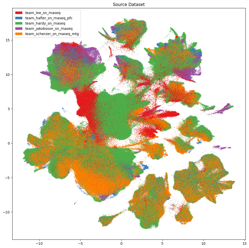
Number of unique source_dataset_label = 5 ['team_hafler_sn_rnaseq_pfc', 'team_hardy_sn_rnaseq', 'team_jakobsson_sn_rnaseq', 'team_lee_sn_rnaseq', 'team_scherzer_sn_rnaseq_mtg']
Number of unique source_dataset_label_order = 5 [1, 2, 3, 4, 5]
Number of unique source_dataset_label_color = 5 ['#377eb8', '#4daf4a', '#984ea3', '#e41a1c', '#ff7f00']
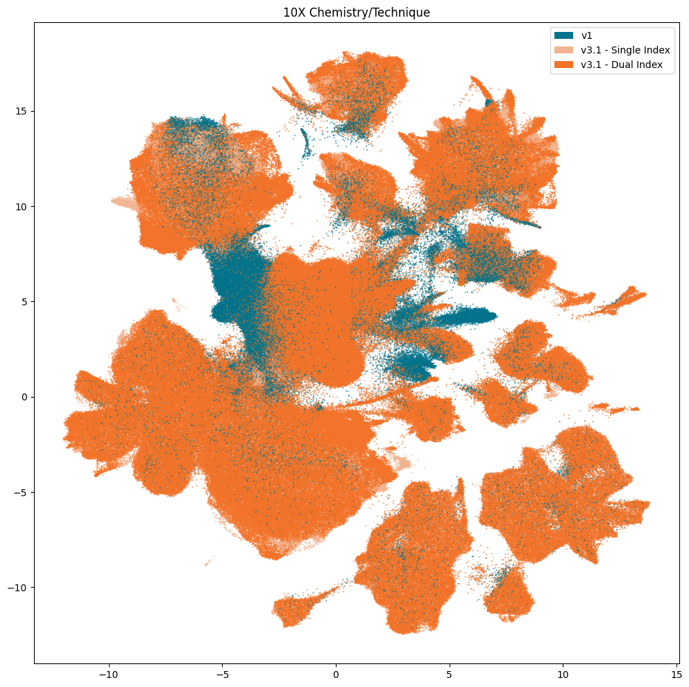
Number of unique technique = 3 ['v1', 'v3.1 - Dual Index', 'v3.1 - Single Index']
Number of unique technique_order = 3 [1, 2, 3]
Number of unique technique_color = 3 ['#03738C', '#F27329', '#F2B591']
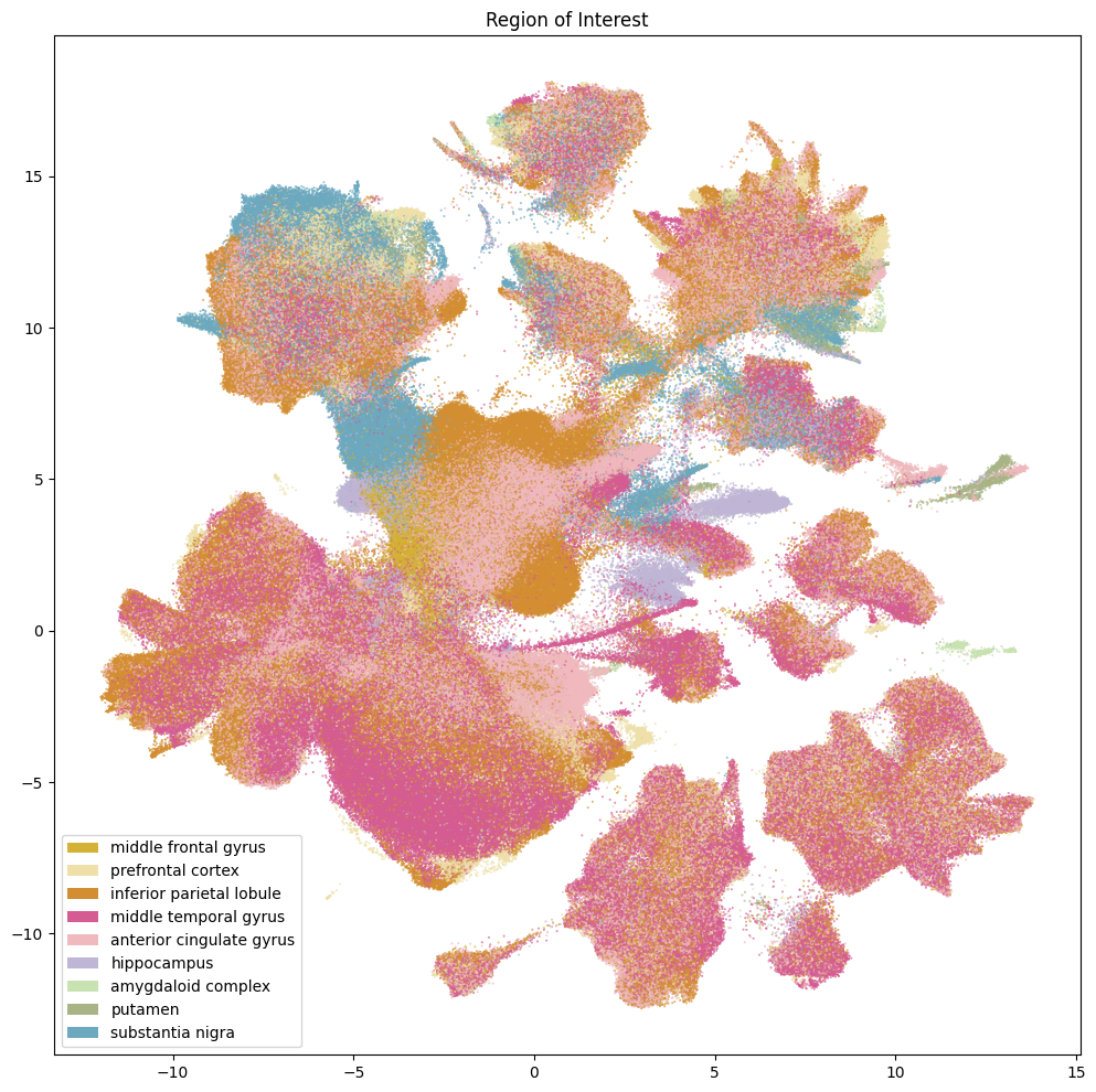
Number of unique region_of_interest_label = 9 ['amygdaloid complex', 'anterior cingulate gyrus', 'hippocampus', 'inferior parietal lobule', 'middle frontal gyrus', 'middle temporal gyrus', 'prefrontal cortex', 'putamen', 'substantia nigra']
Number of unique region_of_interest_label_order = 9 [1, 2, 3, 4, 5, 6, 7, 8, 9]
Number of unique region_of_interest_label_color = 9 ['#6ca9bf', '#a8b485', '#bfb5d5', '#c9e2b1', '#d38e32', '#d4b235', '#d55c92', '#eee0a8', '#efb9be']
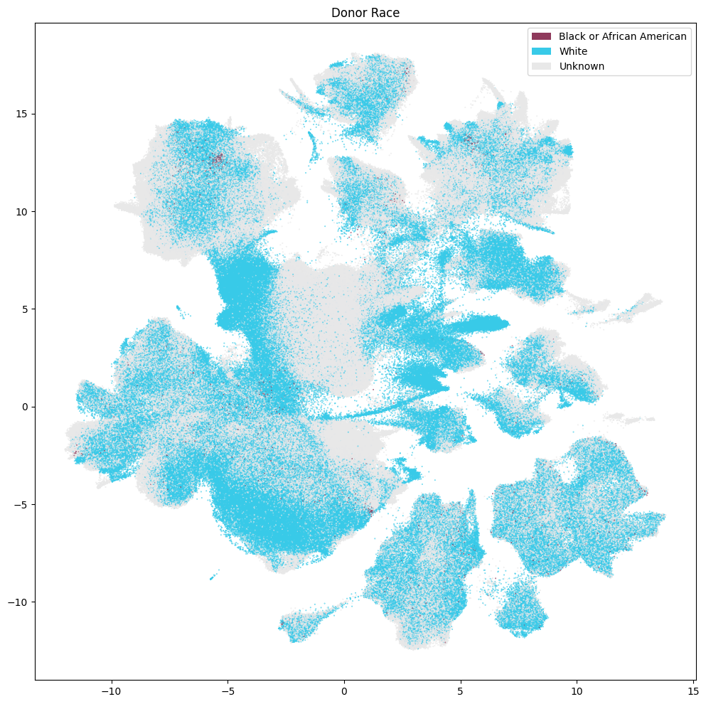
Number of unique donor_race = 3 ['Black or African American', 'Unknown', 'White']
Number of unique donor_race_order = 3 [1, 2, 3]
Number of unique donor_race_color = 3 ['#38CAE8', '#8F3A5C', '#e8e8e8']
Number of unique donor_sex = 2 ['Female', 'Male']
Number of unique donor_sex_order = 2 [1, 2]
Number of unique donor_sex_color = 2 ['#565353', '#ADC4C3']
Number of unique primary_diagnosis = 7 ["Alzheimer's disease", 'Healthy Control', "Idiopathic Parkinson's disease", 'No PD nor other neurological disorder', 'Other neurological disorder', "Parkinson's disease", "Prodromal motor Parkinson's disease"]
Number of unique primary_diagnosis_order = 7 [1, 2, 3, 4, 5, 6, 7]
Number of unique primary_diagnosis_color = 7 ['#3288bd', '#99d594', '#d53e4f', '#e6f598', '#fc8d59', '#fee08b', '#ffffbf']
Number of unique age_at_death = 4 ['65 - 77 yrs', '78 - 89 yrs', '90+ yrs', '< 65 yrs']
Number of unique age_at_death_order = 4 [1, 2, 3, 4]
Number of unique age_at_death_color = 4 ['#2b8cbe', '#7bccc4', '#bae4bc', '#f0f9e8']
Number of unique apoe4_status = 7 ['Unknown', 'e2/e2', 'e2/e3', 'e2/e4', 'e3/e3', 'e3/e4', 'e4/e4']
Number of unique apoe4_status_order = 7 [1, 2, 3, 4, 5, 6, 7]
Number of unique apoe4_status_color = 7 ['#1b9e77', '#66a61e', '#7570b3', '#d95f02', '#e6ab02', '#e7298a', '#e8e8e8']
Number of unique braak_stage = 7 ['Braak 0', 'Braak I', 'Braak II', 'Braak III', 'Braak IV', 'Braak VI', 'Unknown']
Number of unique braak_stage_order = 6 [1, 2, 3, 4, 5, 7]
Number of unique braak_stage_color = 7 ['#91003f', '#c994c7', '#d4b9da', '#df65b0', '#e7298a', '#e8e8e8', '#f1eef6']
Number of unique cerad_score = 4 ['Frequent', 'Moderate', 'Sparse', 'Unknown']
Number of unique cerad_score_order = 4 [1, 2, 3, 4]
Number of unique cerad_score_color = 4 ['#377eb8', '#4daf4a', '#e41a1c', '#e8e8e8']
Number of unique cognitive_status = 4 ['Dementia', 'Mild Cognitive Impairment', 'Normal', 'Unknown']
Number of unique cognitive_status_order = 4 [1, 2, 3, 4]
Number of unique cognitive_status_color = 4 ['#377eb8', '#4daf4a', '#e41a1c', '#e8e8e8']
Number of unique lewy_body_disease_pathology = 10 ['Absent', 'Amygdala predominant', 'Brainstem predominant', 'Brainstem/Limbic', 'Diffuse, neocortical (brainstem, limbic and neocortical involvement)', 'Limbic (transitional)', 'Limbic predominant', 'Neocortical', 'Olfactory bulb only', 'Unknown']
Number of unique lewy_body_disease_pathology_order = 10 [1, 2, 3, 4, 5, 6, 7, 8, 9, 10]
Number of unique lewy_body_disease_pathology_color = 10 ['#081d58', '#1d91c0', '#225ea8', '#253494', '#41b6c4', '#7fcdbb', '#c7e9b4', '#e8e8e8', '#edf8b1', '#ffffd9']
Number of unique thal_phase = 8 ['Thal 0', 'Thal 1', 'Thal 2', 'Thal 3', 'Thal 4', 'Thal 4/5', 'Thal 5', 'Unknown']
Number of unique thal_phase_order = 8 [1, 2, 3, 4, 5, 6, 7, 8]
Number of unique thal_phase_color = 8 ['#91003f', '#c994c7', '#ce1256', '#d4b9da', '#df65b0', '#e7298a', '#e8e8e8', '#f1eef6']

Finally, we’ll load the value_sets table. This is mainly a mapping between the different sets of terms (e.g. regions of interest, cell types, age ranges), providing unique colors for each term in a set and an order of the set. We’ll primarily use it as a lookup table to order or different terms in plot legends.

value_sets = abc_cache.get_metadata_dataframe(
    directory='ASAP-PMDBS-10X',
    file_name='value_sets'
).set_index('label')
value_sets.head()

value_sets.csv: 100%|████████████████████████████████████████████████████████████████████████| 4.25k/4.25k [00:00<00:00, 71.3kMB/s]

	field	order	color_hex_triplet
label
v1	technique	1	#03738C
v3.1 - Dual Index	technique	3	#F27329
v3.1 - Single Index	technique	2	#F2B591
cluster_000	cluster_label	1	#171c97
cluster_001	cluster_label	2	#e4a9ba

UMAP Plotting

We define convenience function to plot the Uniform Manifold Approximation and Projection (UMAP) of the ASAP PMDB data.

def plot_umap(
    xx,
    yy,
    cc=None,
    val=None,
    fig_width=8,
    fig_height=8,
    cmap=None,
    labels=None,
    term_order_lookup=None,
    colorbar=False,
    sizes=None
):
    """
    """
    if sizes is None:
        sizes = 1
    fig, ax = plt.subplots()
    fig.set_size_inches(fig_width, fig_height)

    if cmap is not None:
        scatt = ax.scatter(xx, yy, c=val, s=0.5, marker='.', cmap=cmap, alpha=sizes)
    elif cc is not None:
        scatt = ax.scatter(xx, yy, c=cc, s=0.5, marker='.', alpha=sizes)

    if labels is not None:
        from matplotlib.patches import Rectangle
        unique_labels = labels.unique()
        unique_colors = cc.unique()

        if term_order_lookup is not None:
            term_order = np.argsort(term_order_lookup.loc[unique_labels, 'order'])
            unique_labels = unique_labels[term_order]
            unique_colors = unique_colors[term_order]
            
        rects = []
        for color in unique_colors:
            rects.append(Rectangle((0, 0), 1, 1, fc=color))

        legend = ax.legend(rects, unique_labels, loc=0)
        # ax.add_artist(legend)

    if colorbar:
        fig.colorbar(scatt, ax=ax)
    
    return fig, ax

Data Acquisition Metadata

Below we plot various information associated with the collection of the data. This includes which of the five teams collected the data, the 10X chemistry version used, and the region of interest the tissue was extracted from. Note, throughout the presentation of these data, that some values are missing for collections of cells. This is due to the value not being present for these cells and samples in the data. These are marked as Unknown.

fig, ax = plot_umap(
    cell_metadata['x'],
    cell_metadata['y'],
    cc=cell_metadata['source_dataset_label_color'],
    labels=cell_metadata['source_dataset_label'],
    term_order_lookup=value_sets,
    fig_width=12,
    fig_height=12
)
res = ax.set_title("Source Dataset")
plt.show()

fig, ax = plot_umap(
    cell_metadata['x'],
    cell_metadata['y'],
    cc=cell_metadata['technique_color'],
    labels=cell_metadata['technique'],
    term_order_lookup=value_sets,
    fig_width=12,
    fig_height=12
)
res = ax.set_title("10X Chemistry/Technique")
plt.show()

fig, ax = plot_umap(
    cell_metadata['x'],
    cell_metadata['y'],
    cc=cell_metadata['region_of_interest_label_color'],
    labels=cell_metadata['region_of_interest_label'],
    term_order_lookup=value_sets,
    fig_width=12,
    fig_height=12
)
res = ax.set_title("Region of Interest")
plt.show()

Donor Metadata

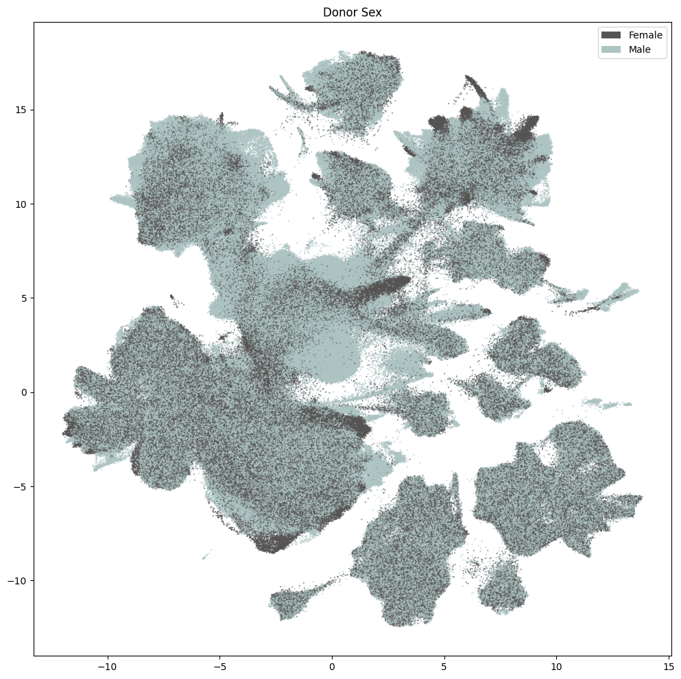
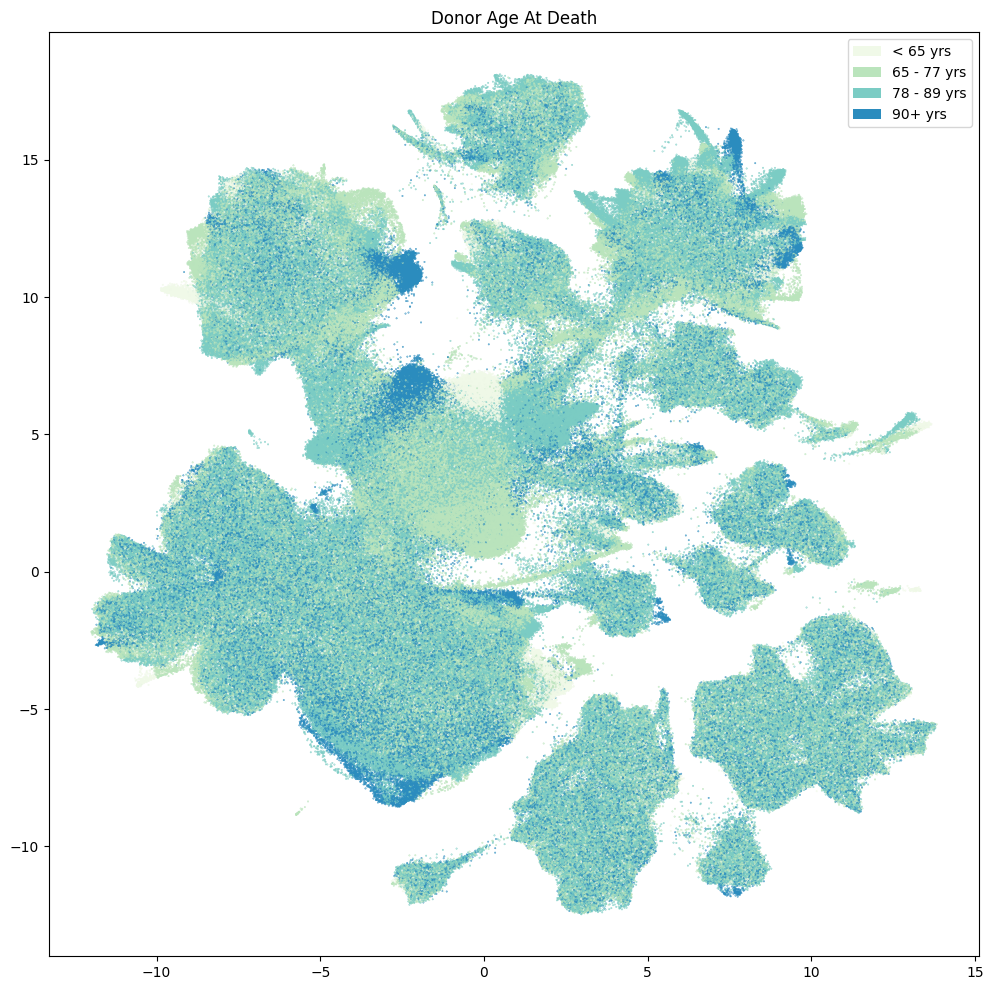
Below we plot various information on the donor where these samples/cells originated.

fig, ax = plot_umap(
    cell_metadata['x'],
    cell_metadata['y'],
    cc=cell_metadata['donor_race_color'],
    labels=cell_metadata['donor_race'],
    term_order_lookup=value_sets[value_sets['field'] == 'donor_race'],
    fig_width=12,
    fig_height=12
)
res = ax.set_title("Donor Race")
plt.show()

fig, ax = plot_umap(
    cell_metadata['x'],
    cell_metadata['y'],
    cc=cell_metadata['donor_sex_color'],
    labels=cell_metadata['donor_sex'],
    term_order_lookup=value_sets[value_sets['field'] == 'donor_sex'],
    fig_width=12,
    fig_height=12
)
res = ax.set_title("Donor Sex")
plt.show()

fig, ax = plot_umap(
    cell_metadata['x'],
    cell_metadata['y'],
    cc=cell_metadata['age_at_death_color'],
    labels=cell_metadata['age_at_death'],
    term_order_lookup=value_sets[value_sets['field'] == 'age_at_death'],
    fig_width=12,
    fig_height=12
)
res = ax.set_title("Donor Age At Death")
plt.show()

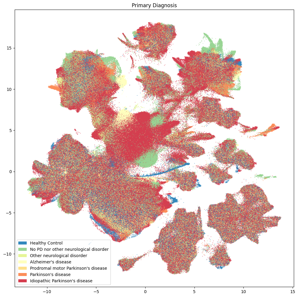
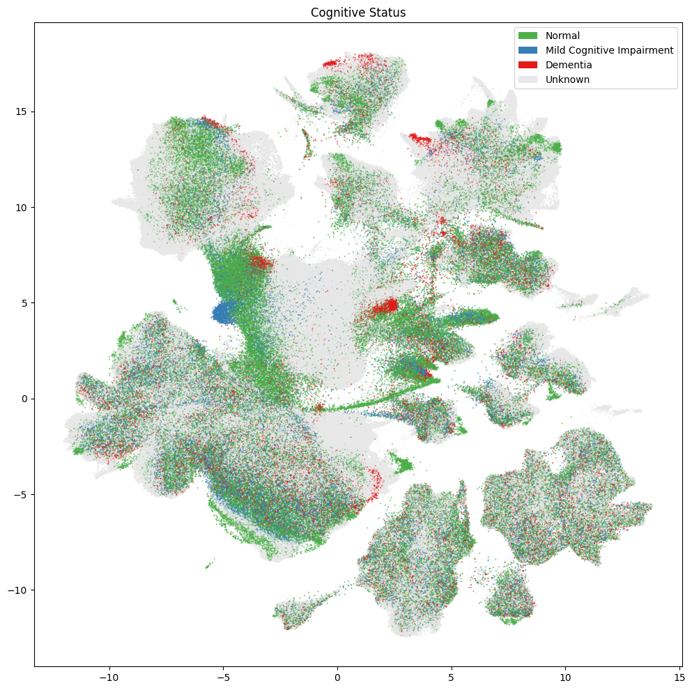
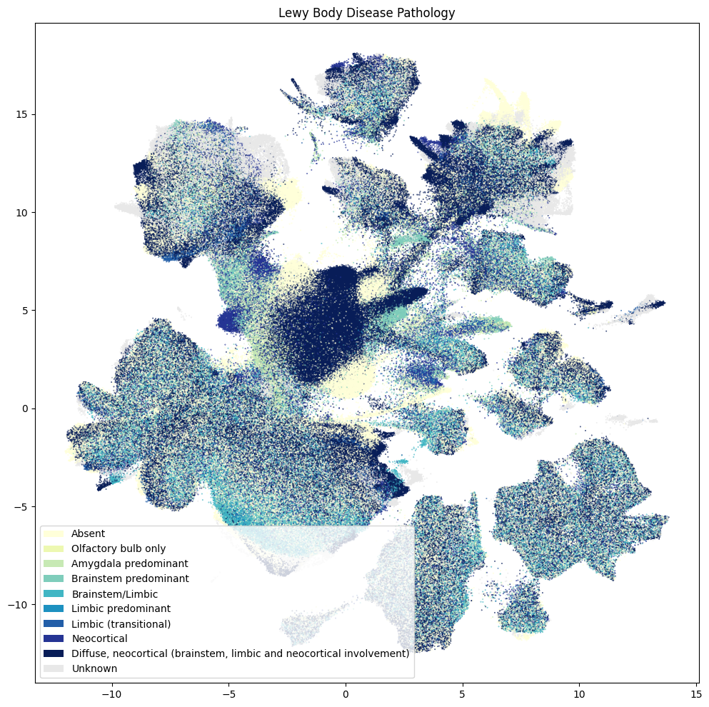
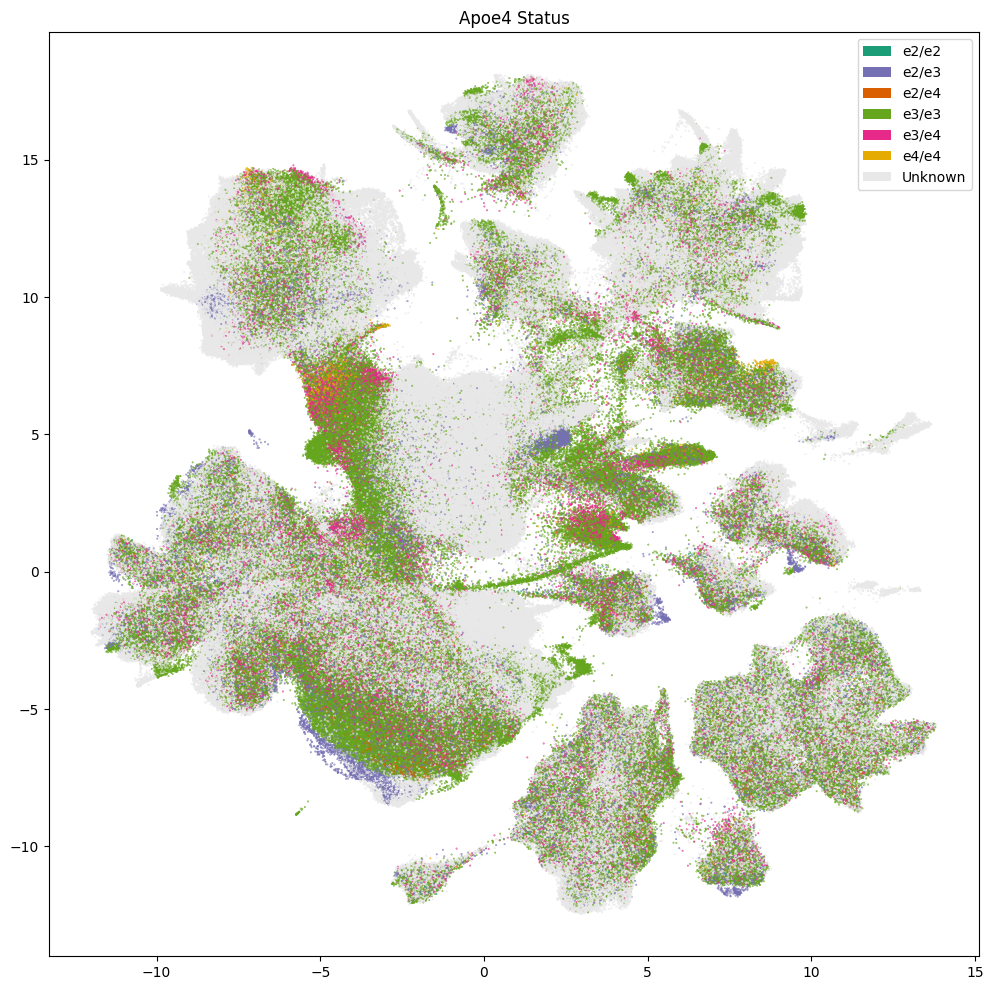
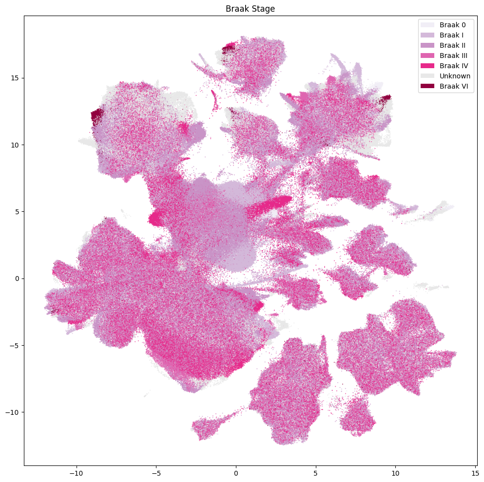
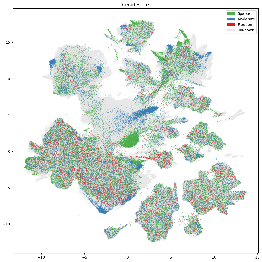
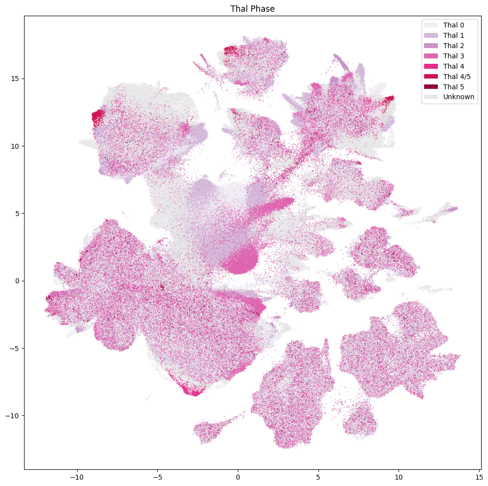
Clinical Pathology

Below are various diagnoses and pathologies identified in the donor including healthy controls.

fig, ax = plot_umap(
    cell_metadata['x'],
    cell_metadata['y'],
    cc=cell_metadata['primary_diagnosis_color'],
    labels=cell_metadata['primary_diagnosis'],
    term_order_lookup=value_sets[value_sets['field'] == 'primary_diagnosis'],
    fig_width=12,
    fig_height=12
)
res = ax.set_title("Primary Diagnosis")
plt.show()

fig, ax = plot_umap(
    cell_metadata['x'],
    cell_metadata['y'],
    cc=cell_metadata['cognitive_status_color'],
    labels=cell_metadata['cognitive_status'],
    term_order_lookup=value_sets[value_sets['field'] == 'cognitive_status'],
    fig_width=12,
    fig_height=12
)
res = ax.set_title("Cognitive Status")
plt.show()

fig, ax = plot_umap(
    cell_metadata['x'],
    cell_metadata['y'],
    cc=cell_metadata['lewy_body_disease_pathology_color'],
    labels=cell_metadata['lewy_body_disease_pathology'],
    term_order_lookup=value_sets[value_sets['field'] == 'lewy_body_disease_pathology'],
    fig_width=12,
    fig_height=12
)
res = ax.set_title("Lewy Body Disease Pathology")
plt.show()

fig, ax = plot_umap(
    cell_metadata['x'],
    cell_metadata['y'],
    cc=cell_metadata['apoe4_status_color'],
    labels=cell_metadata['apoe4_status'],
    term_order_lookup=value_sets[value_sets['field'] == 'apoe4_status'],
    fig_width=12,
    fig_height=12
)
res = ax.set_title("Apoe4 Status")
plt.show()

fig, ax = plot_umap(
    cell_metadata['x'],
    cell_metadata['y'],
    cc=cell_metadata['braak_stage_color'],
    labels=cell_metadata['braak_stage'],
    term_order_lookup=value_sets[value_sets['field'] == 'braak_stage'],
    fig_width=12,
    fig_height=12
)
res = ax.set_title("Braak Stage")
plt.show()

fig, ax = plot_umap(
    cell_metadata['x'],
    cell_metadata['y'],
    cc=cell_metadata['cerad_score_color'],
    labels=cell_metadata['cerad_score'],
    term_order_lookup=value_sets[value_sets['field'] == 'cerad_score'],
    fig_width=12,
    fig_height=12
)
res = ax.set_title("Cerad Score")
plt.show()

fig, ax = plot_umap(
    cell_metadata['x'],
    cell_metadata['y'],
    cc=cell_metadata['thal_phase_color'],
    labels=cell_metadata['thal_phase'],
    term_order_lookup=value_sets[value_sets['field'] == 'thal_phase'],
    fig_width=12,
    fig_height=12
)
res = ax.set_title("Thal Phase")
plt.show()

Leiden scVI Clusters

As part of the ASAP harmonization, scVI was used to generate a latent space representation, 2D UMAP coordinates and set of 30 clusters using their implementation of the Leiden algorithm.

fig, ax = plot_umap(
    cell_metadata['x'],
    cell_metadata['y'],
    cc=cell_metadata['cluster_label_color'],
    fig_width=12,
    fig_height=12
)
res = ax.set_title("Cluster Label")
plt.show()

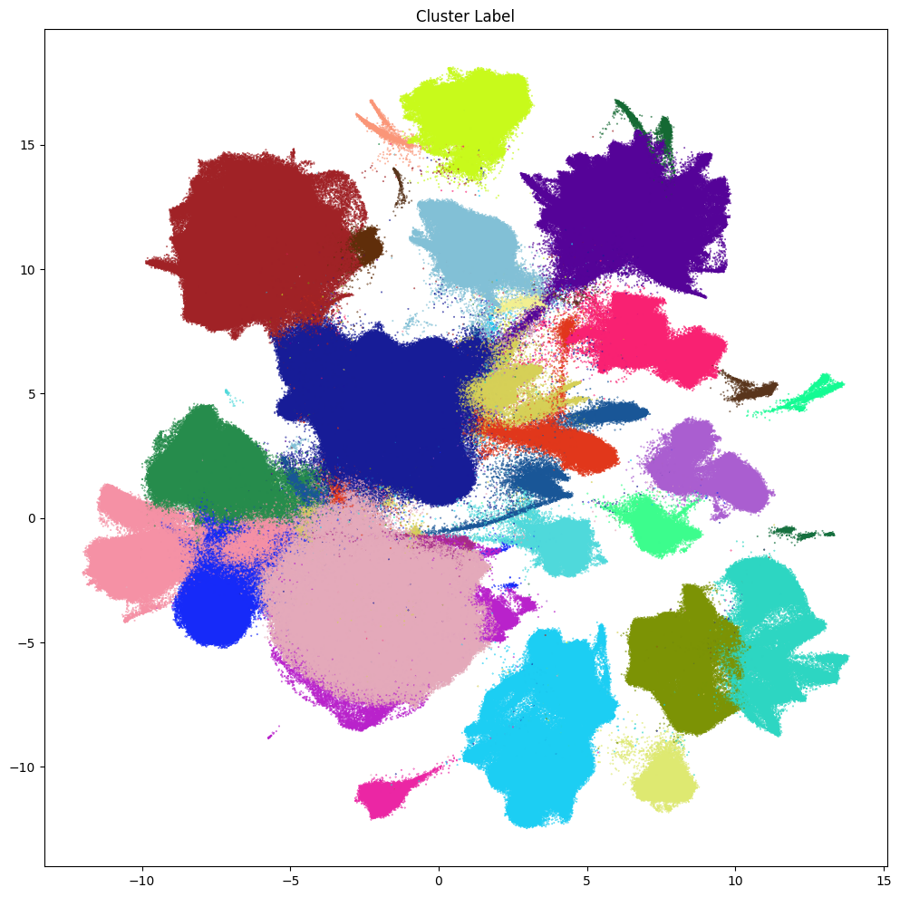
In the next notebook, we demonstrate the usage of Allen Institute’s MapMyCells tool to map cells from the ASAP PMDBS dataset to the whole human brain taxonomy (Siletti et al.) to provide cell type annotation and insights to the Leiden scVI clusters above.

We’ll also explore gene expression in the UMAP in a later notebook.