Whole Human Brain 10x RNA-seq clustering analysis and annotation

The Whole Human Brain Atlas data 10X RNA-seq dataset contains ~3 million nuclei (more than 2 million sequenced neurons and almost 1 million non-neurons) from 100 locations across the forebrain, midbrain, and hindbrain. The integrated transcriptomic taxonomy contains 31 superclusters, 461 clusters, and 3313 subclusters. Full details of the dataset can be found in Siletti et al. 2023

The purpose of this notebook is to provide an overview of how cluster and cluster annotation information is represented through example use cases. Note that cluster in this notebook is an overloaded term as one of the levels is referred to as cluster while it can also refer to the general clustering of similar cells.

You need to be connected to the internet to run this notebook and that you have already downloaded the data via the getting started notebook.

import os
import pandas as pd
import numpy as np
import matplotlib.pyplot as plt
from pathlib import Path

from abc_atlas_access.abc_atlas_cache.abc_project_cache import AbcProjectCache

We will interact with the data using the AbcProjectCache. This cache object tracks which data has been downloaded and serves the path to the requsted data on disk. For metadata, the cache can also directly serve a up a Pandas Dataframe. See the getting_started notebook for more details on using the cache including installing it if it has not already been.

Change the download_base variable to where you have downloaded the data in your system.

download_base = Path('../../abc_download_root')
abc_cache = AbcProjectCache.from_s3_cache(download_base)
abc_cache.current_manifest

'releases/20240330/manifest.json'

Data Overview

Below we list the available metadata in the WHB-taxonomy directory.

abc_cache.list_metadata_files('WHB-taxonomy')

['cluster',
 'cluster_annotation_term',
 'cluster_annotation_term_set',
 'cluster_to_cluster_annotation_membership']

Subclusters

Each of the final set of 3313 subclusters is associated with an alias and label. Each row of the dataframe represents a subcluster as defined in Siletti et al. 2023. Each subcluster has a label (string that is unique in the database), cluster alias (in this case a simple integer) and the number of cells that has been grouped into the cluster.

cluster = abc_cache.get_metadata_dataframe(directory='WHB-taxonomy', file_name='cluster')
print(len(cluster))
cluster

cluster.csv: 100%|██████████| 84.8k/84.8k [00:00<00:00, 433kMB/s] 

3313

	cluster_alias	number_of_cells	label
0	0	34	CS202210140_494
1	1	220	CS202210140_495
2	2	187	CS202210140_496
3	3	246	CS202210140_497
4	4	188	CS202210140_498
...	...	...	...
3308	3308	140	CS202210140_3802
3309	3309	138	CS202210140_3803
3310	3310	85	CS202210140_3804
3311	3311	93	CS202210140_3805
3312	3312	74	CS202210140_3806

3313 rows × 3 columns

Cluster annotation term sets

Each level of classification is represented as a cluster annotation term set. Each term set consists of a set of ordered terms. Each term set has a label (human readable string that is unique in the database), a name, description and order among the term sets.

term_set = abc_cache.get_metadata_dataframe(directory='WHB-taxonomy', file_name='cluster_annotation_term_set')
term_set

	label	name	description	order
0	CCN202210140_SUBC	subcluster	The finest level of cell type definition in th...	2
1	CCN202210140_CLUS	cluster	An intermediate level of cell type definitions...	1
2	CCN202210140_SUPC	supercluster	The top level of cell type definition in the h...	0
3	CCN202210140_NEUR	neurotransmitter	Neurotransmitter terms are assigned to cluster...	3

We can use the pandas iterrows function to print out the description for each term set.

# print out description for each term_set
for tsindex, tsrow in term_set.iterrows():
    print("%s:\n" % tsrow['name'])
    print("%s\n" % tsrow['description'])

subcluster:

The finest level of cell type definition in the human whole brain taxonomy. It is defined by applying Louvain clustering independently for each cluster. Cells within a subcluster share similar characteristics and belong to the same cluster. In some cases subclusters are distinct, and in other cases represent cell states or gradients within the same cluster.

cluster:

An intermediate level of cell type definitions in the human whole brain taxonomy. It is defined by applying Louvain clustering independently for each supercluster. All cells within a subcluster belong to the same cluster.   Clusters group together similar subclusters and are highly distinct from one another.

supercluster:

The top level of cell type definition in the human whole brain taxonomy. It is defined using Louvain clustering (Cytograph) with most superclusters determined by broad brain region and neurotransmitter type.  All cells within a cluster belong to the same supercluster. Supercluster provides a broader characterization of cell types.

neurotransmitter:

Neurotransmitter terms are assigned to clusters based on the expression (or lack of expression) of one or more neurotransmitter-associated transporter or enzyme genes

Cluster annotation terms

A cluster annotation term represents a group within a single level of classification. Each term object has a label (human readable string that is unique in the database), a name, which cluster annotation term set it belongs to and a parent or superclass if the term forms a hierarchy, an order within a term set and a color for visualization purposes.

term = abc_cache.get_metadata_dataframe(directory='WHB-taxonomy', file_name='cluster_annotation_term', keep_default_na=False)
term.head(5)

cluster_annotation_term.csv: 100%|██████████| 547k/547k [00:00<00:00, 2.87MMB/s] 

	label	name	cluster_annotation_term_set_label	parent_term_label	parent_term_set_label	term_set_order	term_order	cluster_annotation_term_set_name	color_hex_triplet	number_of_cells	description
0	CS202210140_476	Upper-layer intratelencephalic	CCN202210140_SUPC			0	0	supercluster	#FEA7BA	455006	Upper-layer intratelencephalic
1	CS202210140_477	Deep-layer intratelencephalic	CCN202210140_SUPC			0	1	supercluster	#426600	228467	Deep-layer intratelencephalic
2	CS202210140_473	Deep-layer near-projecting	CCN202210140_SUPC			0	2	supercluster	#EE1010	18856	Deep-layer near-projecting
3	CS202210140_474	Deep-layer corticothalamic and 6b	CCN202210140_SUPC			0	3	supercluster	#5EF0F1	78396	Deep-layer corticothalamic and 6b
4	CS202210140_484	MGE interneuron	CCN202210140_SUPC			0	4	supercluster	#DFFE66	222434	MGE interneuron

We can use the groupby and count functions in pandas to tally the number of terms in each term set (classification level).

term[['label','cluster_annotation_term_set_name']].groupby('cluster_annotation_term_set_name').count()

	label
cluster_annotation_term_set_name
cluster	461
neurotransmitter	20
subcluster	3313
supercluster	31

Unlike the Whole Mouse brain data, the term names are unique across term sets.

Cluster to cluster annotation membership

The association between a subcluster and cluster annotation term is represented as a cluster to cluster annotation membership within the context of one cluster annotation term set. It is expected that a cluster in only associated with one term within a specific term set.

membership = abc_cache.get_metadata_dataframe(directory='WHB-taxonomy', file_name='cluster_to_cluster_annotation_membership')
membership.head(5)

	cluster_annotation_term_label	cluster_annotation_term_set_label	cluster_alias	cluster_annotation_term_name	cluster_annotation_term_set_name	number_of_cells	color_hex_triplet
0	CS202210140_494	CCN202210140_SUBC	0	URL_297_0	subcluster	34	#7E807A
1	CS202210140_495	CCN202210140_SUBC	1	URL_308_1	subcluster	220	#C54945
2	CS202210140_496	CCN202210140_SUBC	2	URL_308_2	subcluster	187	#5232B7
3	CS202210140_497	CCN202210140_SUBC	3	URL_308_3	subcluster	246	#31BEBA
4	CS202210140_498	CCN202210140_SUBC	4	URL_308_4	subcluster	188	#C8A9BC

Example use cases

Aggregating cluster and cells counts per term

We can obtain cluster and cell counts per cluster annotation term using the pandas groupby function.

# Count the number of clusters associated with each cluster annotation term
term_cluster_count = membership.groupby(['cluster_annotation_term_label'])[['cluster_alias']].count()
term_cluster_count.columns = ['number_of_clusters']
term_cluster_count.head(5)

	number_of_clusters
cluster_annotation_term_label
CS202210140_1	1
CS202210140_10	2
CS202210140_100	9
CS202210140_1000	1
CS202210140_1001	1

# Join counts with the term dataframe
term_by_label = term.set_index('label')
term_with_counts = term_by_label.join(term_cluster_count)
term_with_counts[['name', 'cluster_annotation_term_set_name', 'number_of_clusters', 'number_of_cells']].head(5)

	name	cluster_annotation_term_set_name	number_of_clusters	number_of_cells
label
CS202210140_476	Upper-layer intratelencephalic	supercluster	139	455006
CS202210140_477	Deep-layer intratelencephalic	supercluster	138	228467
CS202210140_473	Deep-layer near-projecting	supercluster	72	18856
CS202210140_474	Deep-layer corticothalamic and 6b	supercluster	116	78396
CS202210140_484	MGE interneuron	supercluster	211	222434

Let’s visualize cluster and cells counts for of the classification levels using bar plots.

def bar_plot_by_level_and_type(df, level, fig_width = 8.5, fig_height = 4):
    
    fig, ax = plt.subplots(1, 2)
    fig.set_size_inches(fig_width, fig_height)
    
    for idx, ctype in enumerate(['clusters', 'cells']):

        pred = (df['cluster_annotation_term_set_name'] == level)
        names = df[pred]['name']
        counts = df[pred]['number_of_%s' % ctype]
        colors = df[pred]['color_hex_triplet']
        
        ax[idx].barh(names, counts, color=colors)
        ax[idx].set_title('Number of %s by %s' % (ctype,level)),
        ax[idx].set_xscale('log')
        
        if idx > 0:
            ax[idx].set_yticklabels([])

    plt.show()

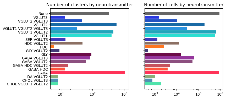
Neurotransmitter cluster and cell counts

The majority of clusters and cells are of glutamatergic, GABAergic or GABA-glycinergic neurotransmitter types.

df = term_with_counts
level = 'neurotransmitter'
pred = (df['cluster_annotation_term_set_name'] == level)

bar_plot_by_level_and_type(term_with_counts, 'neurotransmitter')

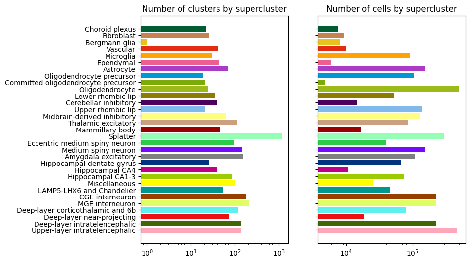
Supercluster level cluster and cell counts

Supercluster “Splatter” contains the largest number of subclusters (~1k), while “Oligodendrocyte” and “Upper-layer intratelencephalic” have the most cells.

bar_plot_by_level_and_type(term_with_counts, 'supercluster', 8.5, 6)

Visualizing cluster and term distributions

We can explore the relationship and distribution of clusters between term sets by creating a pivot table using pandas groupby fuunction. Each row of the resulting dataframe represents a cluster, each column represents a term set and the value in the table is the name of the term that has been associated with the cluster for that specific term set.

pivot = membership.groupby(['cluster_alias', 'cluster_annotation_term_set_name'])['cluster_annotation_term_name'].first().unstack()
pivot = pivot[term_set['name']] # order columns
pivot

cluster_annotation_term_set_name	subcluster	cluster	supercluster	neurotransmitter
cluster_alias
0	URL_297_0	URL_297	Upper rhombic lip	VGLUT1
1	URL_308_1	URL_308	Upper rhombic lip	VGLUT1
2	URL_308_2	URL_308	Upper rhombic lip	VGLUT1
3	URL_308_3	URL_308	Upper rhombic lip	VGLUT1
4	URL_308_4	URL_308	Upper rhombic lip	VGLUT1
...	...	...	...	...
3308	Nkcell_2_3308	Nkcell_2	Miscellaneous	None
3309	Nkcell_2_3309	Nkcell_2	Miscellaneous	None
3310	Nkcell_2_3310	Nkcell_2	Miscellaneous	None
3311	Nkcell_2_3311	Nkcell_2	Miscellaneous	None
3312	Nkcell_2_3312	Nkcell_2	Miscellaneous	None

3313 rows × 4 columns

We can also obtain a cluster annotation color pivot table in the same way.

color = membership.groupby(['cluster_alias', 'cluster_annotation_term_set_name'])['color_hex_triplet'].first().unstack().fillna('#f9f9f9')
color = color[term_set['name']] # order columns
color.columns = ['%s_color' % x for x in color.columns]
color

	subcluster_color	cluster_color	supercluster_color	neurotransmitter_color
cluster_alias
0	#7E807A	#909FF6	#80BAED	#2BDFD1
1	#C54945	#A5B0D9	#80BAED	#2BDFD1
2	#5232B7	#A5B0D9	#80BAED	#2BDFD1
3	#31BEBA	#A5B0D9	#80BAED	#2BDFD1
4	#C8A9BC	#A5B0D9	#80BAED	#2BDFD1
...	...	...	...	...
3308	#3D84BA	#E2EE30	#FEFE00	#666666
3309	#C25347	#E2EE30	#FEFE00	#666666
3310	#B9BFB4	#E2EE30	#FEFE00	#666666
3311	#6CC93D	#E2EE30	#FEFE00	#666666
3312	#423149	#E2EE30	#FEFE00	#666666

3313 rows × 4 columns

For a given pair of term sets A and B, define a function distribution that creates a cluster count table where the rows are terms in term set A, columns are terms in term set B and the table values being the number of clusters that is shared between the terms.

def distribution(A, B):
    
    AxB = pivot.groupby([A, B])[['cluster']].count()
    AxB.columns = ['number_of_clusters']
    AxB = AxB.unstack().fillna(0)

    B_names = [x[1] for x in list(AxB.columns)]
    pred = (term['cluster_annotation_term_set_name'] == B)
    term_by_name = term[pred].set_index('name')
    B_colors = term_by_name.loc[B_names, 'color_hex_triplet']
    
    return AxB, B_names, B_colors

Function stacked_bar_distribution takes the results of distribution as input to create distribution stacked bar plot.

def stacked_bar_distribution(AxB, B_names, B_colors, fig_width = 6, fig_height = 6):

    fig, ax = plt.subplots()
    fig.set_size_inches(fig_width, fig_height)

    bottom = np.zeros(len(AxB))

    for i, col in enumerate(AxB.columns):
        ax.barh(AxB.index, AxB[col], left=bottom, label=col[1], color=B_colors[i])
        bottom += np.array(AxB[col])

    ax.set_title('Distribution of %s in each %s' % (AxB.columns.names[1], AxB.index.name))
    ax.legend(loc='center left', bbox_to_anchor=(1, 0.5))

    plt.show()
    
    return fig, ax

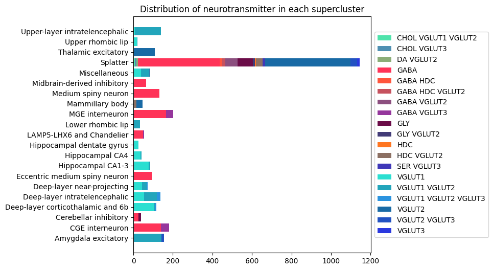
Distribution of neurotransmitter superclusters

Here is the distribution of neurotransmitter types at the supercluster level. Most contain more than one type with splatter showing the most diversity of neurotransmitter types.

AxB, B_names, B_colors = distribution('supercluster', 'neurotransmitter')
fig, ax = stacked_bar_distribution(AxB, B_names, B_colors, 6, 6)

/var/folders/kc/7glrmt5n67x16yj_tg86t49c0000gp/T/ipykernel_15202/1772253940.py:9: FutureWarning: Series.__getitem__ treating keys as positions is deprecated. In a future version, integer keys will always be treated as labels (consistent with DataFrame behavior). To access a value by position, use `ser.iloc[pos]`
  ax.barh(AxB.index, AxB[col], left=bottom, label=col[1], color=B_colors[i])

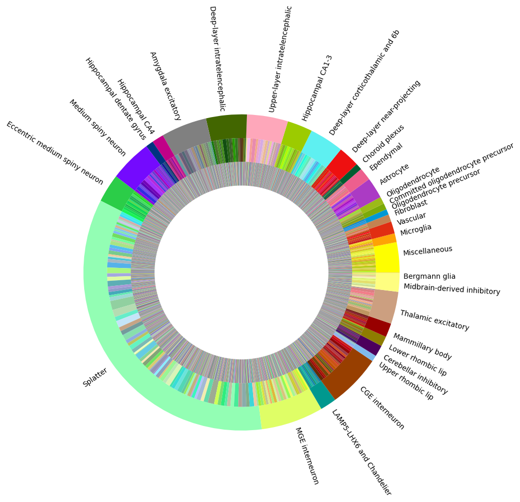
Visualizing the human whole brain taxonomy

Term sets: supercluster, cluster, and subcluster forms a three level human whole brain taxonomy. We can visualized the taxonomy as a sunburst diagram that shows the single inheritance hierarchy through a series of rings, that are sliced for each annotation term. Each ring corresponds to a level in the hierarchy. We have ordered the rings so that the supercluster level is the outer most ring so that we can add in labels. Rings are sliced up and divided based on their hierarchical relationship to the parent slice. The angle of each slice is proportional to the number of clusters belonging to the term.

levels = ['supercluster', 'cluster', 'subcluster']
df = {}

for lvl in levels :
    pred = term_with_counts['cluster_annotation_term_set_name'] == lvl
    df[lvl] = term_with_counts[pred]
    df[lvl] = df[lvl].sort_values(['parent_term_label', 'label'])

fig, ax = plt.subplots()
fig.set_size_inches(10, 10)
size = 0.15

for i, lvl in enumerate(levels):
    
    if lvl == 'supercluster' :
        ax.pie(df[lvl]['number_of_clusters'],
               colors=df[lvl]['color_hex_triplet'],
               labels = df[lvl]['name'],
               rotatelabels=True,
               labeldistance=1.025,
               radius=1,
               wedgeprops=dict(width=size, edgecolor=None),
               startangle=0)
    else :
        ax.pie(df[lvl]['number_of_clusters'],
               colors=df[lvl]['color_hex_triplet'],
               radius=1-i*size,
               wedgeprops=dict(width=size, edgecolor=None),
               startangle=0)

plt.show()