SEA-AD CaH: 10X gene expression

In this notebook we’ll explore gene expressions and combine them with the cell metadata we showed in the previous clustering analysis tutorial.

You need to be connected to the internet to run this notebook or connected to a cache that has the SEA-AD-CaH-10X data downloaded already.

The notebook presented here shows quick visualizations from precomputed metadata in the atlas. For examples on accessing the expression matrices, specifically selecting genes from expression matrices, see the general Accessing expression data tutorial.

%matplotlib inline

import pandas as pd
import numpy as np
from pathlib import Path
import matplotlib.pyplot as plt
from typing import List, Optional, Tuple

from abc_atlas_access.abc_atlas_cache.abc_project_cache import AbcProjectCache
from abc_atlas_access.abc_atlas_cache.anndata_utils import get_gene_data

We will interact with the data using the AbcProjectCache. This cache object tracks which data has been downloaded and serves the path to the requested data on disk. For metadata, the cache can also directly serve up a Pandas DataFrame. See the getting_started notebook for more details on using the cache including installing it if it has not already been.

Change the download_base variable to where you would like to download the data to your system or a location where a cache is already available.

download_base = Path('../../data/allen-brain-cell-atlas-staging/')
abc_cache = AbcProjectCache.from_cache_dir(
   download_base
)

abc_cache.current_manifest

'releases/20260711/manifest.json'

Below we create the expanded cell metadata as was done previously in the cluster annotation tutorial.

cell_to_cluster_membership = abc_cache.get_metadata_dataframe(
    'SEA-AD-CaH-taxonomy', 'cell_to_cluster_membership'
).set_index('cell_label')
cluster = abc_cache.get_metadata_dataframe(
    'SEA-AD-CaH-taxonomy', 'cluster'
).set_index('label')
cluster_annotation_term = abc_cache.get_metadata_dataframe(
    'SEA-AD-CaH-taxonomy', 'cluster_annotation_term'
).set_index('label')

cluster_annotation_term_set = abc_cache.get_metadata_dataframe(
    directory='SEA-AD-CaH-taxonomy',
    file_name='cluster_annotation_term_set'
).set_index('label')

cluster_to_cluster_annotation_membership = abc_cache.get_metadata_dataframe(
    directory='SEA-AD-CaH-taxonomy',
    file_name='cluster_to_cluster_annotation_membership'
).set_index('cluster_annotation_term_label')

cell_metadata = abc_cache.get_metadata_dataframe('SEA-AD-CaH-10X', 'cell_metadata').set_index('cell_label')
membership_with_cluster_info = cluster_to_cluster_annotation_membership.join(
    cluster.reset_index().set_index('cluster_alias')[['number_of_cells']],
    on='cluster_alias'
)

membership_with_cluster_info = membership_with_cluster_info.join(cluster_annotation_term, rsuffix='_anno_term').reset_index()

membership_groupby = membership_with_cluster_info.groupby(
    ['cluster_alias', 'cluster_annotation_term_set_name']
)

cluster_details = membership_groupby['cluster_annotation_term_name'].first().unstack()
cluster_order = membership_groupby['term_order'].first().unstack()

cluster_colors = membership_groupby['color_hex_triplet'].first().unstack()
cluster_colors = cluster_colors[cluster_annotation_term_set['name']]

cell_extended = cell_metadata.join(cell_to_cluster_membership, how='inner')
cell_extended = cell_extended.join(cluster_details, on='cluster_alias')
cell_extended = cell_extended.join(cluster_colors, on='cluster_alias', rsuffix='_color')
cell_extended = cell_extended.join(cluster_order, on='cluster_alias', rsuffix='_order')

library = abc_cache.get_metadata_dataframe(
    directory='SEA-AD-CaH-10X',
    file_name='library'
).set_index('library_label')
donor = abc_cache.get_metadata_dataframe(
    directory='SEA-AD-CaH-10X',
    file_name='donor'
).set_index('donor_label')
disease = abc_cache.get_metadata_dataframe(
    directory='SEA-AD-CaH-10X',
    file_name='disease'
).set_index('donor_label')

cell_extended = cell_extended.join(library, on='library_label', rsuffix='_lib')
cell_extended = cell_extended.join(donor, on='donor_label', rsuffix='_donor')
cell_extended = cell_extended.join(disease, on='donor_label', rsuffix='_disease')

value_sets = abc_cache.get_metadata_dataframe(
    directory='SEA-AD-CaH-10X',
    file_name='value_sets'
).set_index('label')

def extract_value_set(
        cell_metadata_df: pd.DataFrame,
        input_value_set: pd.DataFrame,
        input_value_set_label: str,
        dataframe_column: Optional[str] = None
    ):
    """Add color and order columns to the cell metadata dataframe based on the input
    value set.

    Columns are added as {input_value_set_label}_color and {input_value_set_label}_order.

    Parameters
    ----------
    cell_metadata_df : pd.DataFrame
        DataFrame containing cell metadata.
    input_value_set : pd.DataFrame
        DataFrame containing the value set information.
    input_value_set_label : str
        The the column name to extract color and order information for. will be added to the cell metadata.
    """
    if dataframe_column is None:
        dataframe_column = input_value_set_label
    cell_metadata_df[f'{dataframe_column}_color'] = input_value_set[
        input_value_set['field'] == input_value_set_label
    ].loc[cell_metadata_df[dataframe_column]]['color_hex_triplet'].values
    cell_metadata_df[f'{dataframe_column}_order'] = input_value_set[
        input_value_set['field'] == input_value_set_label
    ].loc[cell_metadata_df[dataframe_column]]['order'].values

# Add region of interest color and order
extract_value_set(cell_extended, value_sets, 'region_of_interest_label')
# Add disease color and order
extract_value_set(cell_extended, value_sets, 'APOE Genotype')
extract_value_set(cell_extended, value_sets, 'Arteriolosclerosis')
extract_value_set(cell_extended, value_sets, 'Atherosclerosis')
extract_value_set(cell_extended, value_sets, 'Braak')
extract_value_set(cell_extended, value_sets, 'CERAD score')
extract_value_set(cell_extended, value_sets, 'Cognitive Status')
extract_value_set(cell_extended, value_sets, 'LATE')
extract_value_set(cell_extended, value_sets, 'Highest Lewy Body Disease')
extract_value_set(cell_extended, value_sets, 'Overall AD neuropathological Change')
extract_value_set(cell_extended, value_sets, 'Thal')
# Add donor sex/gender color and order
extract_value_set(cell_extended, value_sets, 'donor_sex')
extract_value_set(cell_extended, value_sets, 'donor_gender')
# Add race
extract_value_set(cell_extended, value_sets, 'donor_race')
cell_extended.head()

cell_to_cluster_membership.csv: 100%|██████████| 42.1M/42.1M [00:04<00:00, 9.16MMB/s]  
cluster.csv: 100%|██████████| 1.80k/1.80k [00:00<00:00, 21.8kMB/s]
cluster_annotation_term.csv: 100%|██████████| 12.3k/12.3k [00:00<00:00, 121kMB/s]
cluster_annotation_term_set.csv: 100%|██████████| 222/222 [00:00<00:00, 2.34kMB/s]
cluster_to_cluster_annotation_membership.csv: 100%|██████████| 12.4k/12.4k [00:00<00:00, 86.7kMB/s]
cell_metadata.csv: 100%|██████████| 161M/161M [00:25<00:00, 6.25MMB/s]   
/Users/chris.morrison/src/abc_atlas_access/src/abc_atlas_access/abc_atlas_cache/abc_project_cache.py:643: DtypeWarning: Columns (4) have mixed types. Specify dtype option on import or set low_memory=False.
  return pd.read_csv(path, **kwargs)
library.csv: 100%|██████████| 7.64k/7.64k [00:00<00:00, 90.3kMB/s]
donor.csv: 100%|██████████| 8.67k/8.67k [00:00<00:00, 103kMB/s]
disease.csv: 100%|██████████| 8.13k/8.13k [00:00<00:00, 128kMB/s]
value_sets.csv: 100%|██████████| 15.6k/15.6k [00:00<00:00, 126kMB/s]

	cell_barcode	barcoded_cell_sample_label	library_label	alignment_job_id	doublet_score	umi_count	Used in analysis	donor_label	exp_component_name	feature_matrix_label	...	Overall AD neuropathological Change_color	Overall AD neuropathological Change_order	Thal_color	Thal_order	donor_sex_color	donor_sex_order	donor_gender_color	donor_gender_order	donor_race_color	donor_race_order
cell_label
AAACCCAAGAATCTAG-1336_B04	AAACCCAAGAATCTAG	1336_B04	L8HX_220714_02_B02	1194262311	0.05	64074.0	True	H21.33.004	AAACCCAAGAATCTAG-L8HX_220714_02_B02-1194262311	CaH-10X	...	#fcbba1	1	#fedbcb	1	#ADC4C3	2	#ADC4C3	2	#f7f184	125
AAACCCAAGCACAAAT-1336_B04	AAACCCAAGCACAAAT	1336_B04	L8HX_220714_02_B02	1194262311	0.08	37080.0	True	H21.33.004	AAACCCAAGCACAAAT-L8HX_220714_02_B02-1194262311	CaH-10X	...	#fcbba1	1	#fedbcb	1	#ADC4C3	2	#ADC4C3	2	#f7f184	125
AAACCCAAGGGACTGT-1336_B04	AAACCCAAGGGACTGT	1336_B04	L8HX_220714_02_B02	1194262311	0.14	7534.0	False	H21.33.004	AAACCCAAGGGACTGT-L8HX_220714_02_B02-1194262311	CaH-10X	...	#fcbba1	1	#fedbcb	1	#ADC4C3	2	#ADC4C3	2	#f7f184	125
AAACCCACAATTTCCT-1336_B04	AAACCCACAATTTCCT	1336_B04	L8HX_220714_02_B02	1194262311	0.10	4867.0	True	H21.33.004	AAACCCACAATTTCCT-L8HX_220714_02_B02-1194262311	CaH-10X	...	#fcbba1	1	#fedbcb	1	#ADC4C3	2	#ADC4C3	2	#f7f184	125
AAACCCACAGCAATTC-1336_B04	AAACCCACAGCAATTC	1336_B04	L8HX_220714_02_B02	1194262311	0.00	2399.0	True	H21.33.004	AAACCCACAGCAATTC-L8HX_220714_02_B02-1194262311	CaH-10X	...	#fcbba1	1	#fedbcb	1	#ADC4C3	2	#ADC4C3	2	#f7f184	125

5 rows × 105 columns

Single nucleus transcriptomes

Below we use the convenience function get_gene_data to download and extract specific genes from the gene expression h5ad files. This function can be used to pull expression for the full set of cells or any subset from the set of cell metadata for specific genes. See accessing gene expression data tutorial for more information.

We first load the set of genes for these data.

gene = abc_cache.get_metadata_dataframe(
    directory='SEA-AD-CaH-10X',
    file_name='gene'
).set_index('gene_identifier')
gene.head(5)

gene.csv: 100%|██████████| 1.74M/1.74M [00:00<00:00, 3.62MMB/s]

	gene_symbol	feature_types	genome
gene_identifier
ENSG00000243485	MIR1302-2HG	Gene Expression	GRCh38
ENSG00000237613	FAM138A	Gene Expression	GRCh38
ENSG00000186092	OR4F5	Gene Expression	GRCh38
ENSG00000238009	AL627309.1	Gene Expression	GRCh38
ENSG00000239945	AL627309.3	Gene Expression	GRCh38

Below we list the genes we will use in this notebook and the example method used to load the expression for these specific genes from the h5ad file.

To process and extract the gene expressions for yourself, uncomment the code block below. Warning that this is a large amount of data and may take a significant fraction of time to download. This download action will only need to be performed once, however.

For more details on how to extract specific genes from the data see our accessing gene expression data tutorial

gene_names = ['APOE', 'DRD1', 'DRD2', 'AQP4', 'FLT1', 'MME', 'RELN', 'LRP8']

"""
gene_data = get_gene_data(
    abc_atlas_cache=abc_cache,
    all_cells=cell_metadata,
    all_genes=gene,
    selected_genes=gene_names
)"""

'\ngene_data = get_gene_data(\n    abc_atlas_cache=abc_cache,\n    all_cells=cell_metadata,\n    all_genes=gene,\n    selected_genes=gene_names\n)'

Instead of processing the gene expressions, we load pre-processed files containing the log gene expression for the genes listed above. The expression in the table below are presented as log2(CPM + 1).

gene_data = abc_cache.get_metadata_dataframe(
    directory='SEA-AD-CaH-10X',
    file_name='example_gene_expression'
).set_index('cell_label')
gene_data.head()

example_gene_expression.csv: 100%|██████████| 63.9M/63.9M [00:07<00:00, 8.34MMB/s]  

	LRP8	MME	DRD1	RELN	DRD2	FLT1	AQP4	APOE
cell_label
AAACCCAAGAATCTAG-1336_B04	0.000000	9.551004	0.000000	0.000000	8.967003	0.0	0.0	0.000000
AAACCCAAGCACAAAT-1336_B04	0.000000	7.085803	4.805742	7.759886	0.000000	0.0	0.0	0.000000
AAACCCAAGGGACTGT-1336_B04	0.000000	8.640949	0.000000	0.000000	7.063197	0.0	0.0	0.000000
AAACCCACAATTTCCT-1336_B04	0.000000	7.689756	0.000000	0.000000	0.000000	0.0	0.0	7.689756
AAACCCACAGCAATTC-1336_B04	8.706808	0.000000	8.706808	0.000000	0.000000	0.0	0.0	0.000000

We load and merge the expression into each of our cell metadata.

cell_extended = cell_extended.join(gene_data)

Example use cases

In this section, we show a use case plotting our sets of genes. First we’ll show the gene expression in heatmaps plotted disease metadata and the taxonomy. We’ll then plot the genes in a UMAP.

Heatmap of Average gene expression

The helper function below creates a heatmap showing the relation between various parameters in the combined cell metadata and the genes we loaded.

import matplotlib as mpl

def plot_heatmap(
    df: pd.DataFrame,
    gnames: List[str],
    value: str,
    sort: bool = False,
    fig_width: float = 8,
    fig_height: float = 4,
    vmax: float = None,
    cmap: plt.cm = plt.cm.magma,
):
    """Plot a heatmap of gene expression values for a list of genes across species.

    Parameters
    ----------
    df : pd.DataFrame
        DataFrame containing cell metadata and gene expression values.
    gnames : list
        List of gene names to plot.
    value : str
        Column name in df to group by (e.g., 'species_genus').
    sort : bool, optional
        Whether to sort the gene expression values within each species.
    fig_width : float, optional
        Width of the figure in inches.
    fig_height : float, optional
        Height of the figure in inches.
    vmax : float, optional
        Maximum value for the color scale. If None, it is set to the maximum value in the data.
    cmap : matplotlib colormap, optional
        Colormap to use for the heatmap.

    Returns
    -------
    fig : matplotlib.figure.Figure
        The figure object containing the heatmap.
    ax : array of matplotlib.axes.Axes
        The axes objects for each species.
    """

    fig, ax = plt.subplots(1, 1)
    fig.set_size_inches(fig_width, fig_height)

    grouped = df.groupby(value)[gnames].mean()
    vmin = grouped.min().min()
    vmax = grouped.max().max()
    norm = mpl.colors.Normalize(vmin=vmin, vmax=vmax)
    sm = plt.cm.ScalarMappable(cmap=cmap, norm=norm)
    cmap = sm.get_cmap()

    if sort:
        grouped = grouped.sort_values(by=gnames[0], ascending=False)
        grouped = grouped.loc[sorted(grouped.index)]

    value_order = df.groupby(value)[[f'{value}_order']].first()
    grouped = grouped.loc[
        value_order.sort_values(f'{value}_order').index
    ]

    arr = grouped.to_numpy().astype('float')

    ax.imshow(arr, cmap=cmap, aspect='auto', vmin=vmin, vmax=vmax)
    xlabs = grouped.columns.values
    ylabs = grouped.index.values


    ax.set_yticks(range(len(ylabs)))
    ax.set_yticklabels(ylabs)
    ax.set_xticks(range(len(xlabs)))
    ax.set_xticklabels(xlabs)

    cbar = fig.colorbar(sm, ax=ax, orientation='vertical', fraction=0.01, pad=0.01)
    cbar.set_label('Mean Expression [log2(CPM + 1)]')
    plt.subplots_adjust(wspace=0.00, hspace=0.00)
    
    return fig, ax

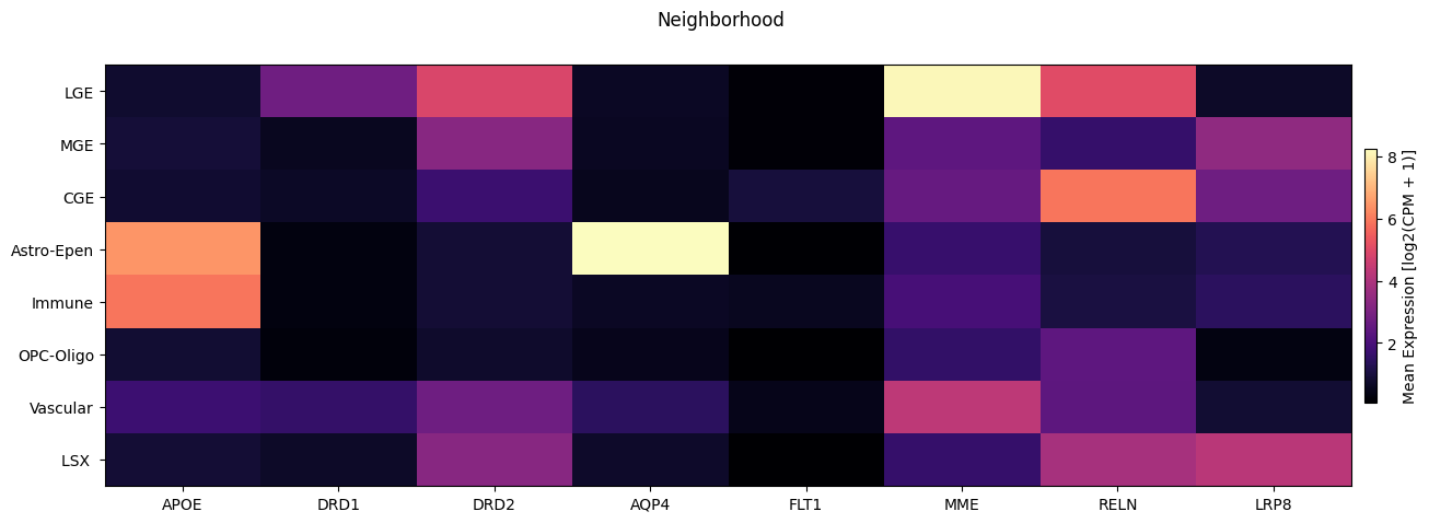
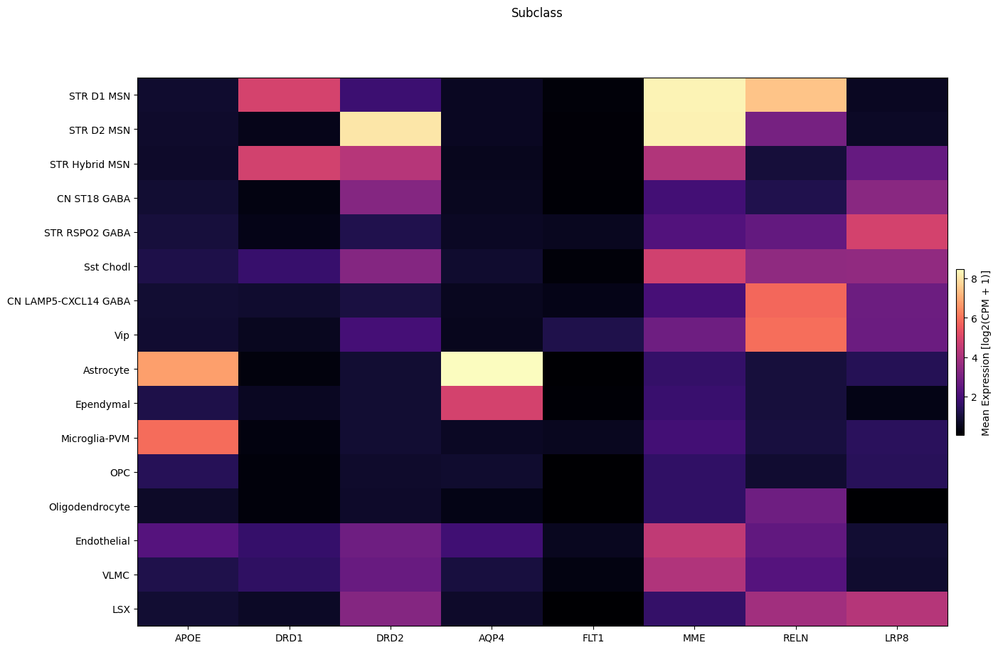
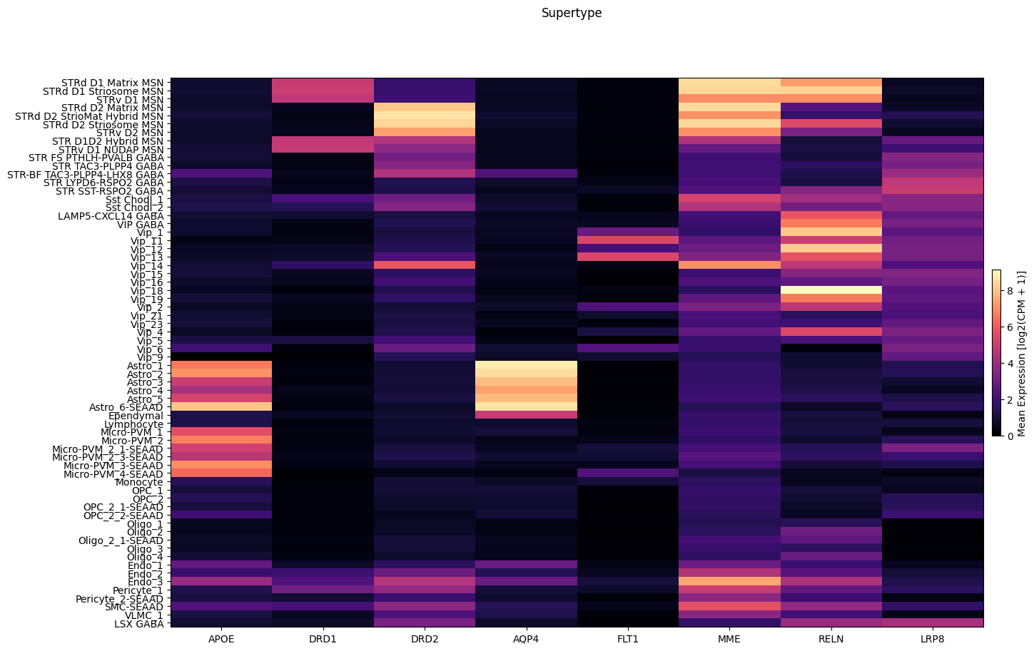
We now use the above function to show the average expression across neighborhood, subclass, and supertype.

fig, ax = plot_heatmap(
    df=cell_extended,
    gnames=gene_names,
    value='Neighborhood',
    fig_width=15,
    fig_height=5
)
fig.suptitle('Neighborhood')
plt.show()

fig, ax = plot_heatmap(
    df=cell_extended,
    gnames=gene_names,
    value='Subclass',
    fig_width=15,
    fig_height=10,
    sort=True
)
fig.suptitle('Subclass')
plt.show()

fig, ax = plot_heatmap(
    df=cell_extended,
    gnames=gene_names,
    value='Supertype',
    fig_width=15,
    fig_height=10,
    sort=True
)
fig.suptitle('Supertype')
plt.show()

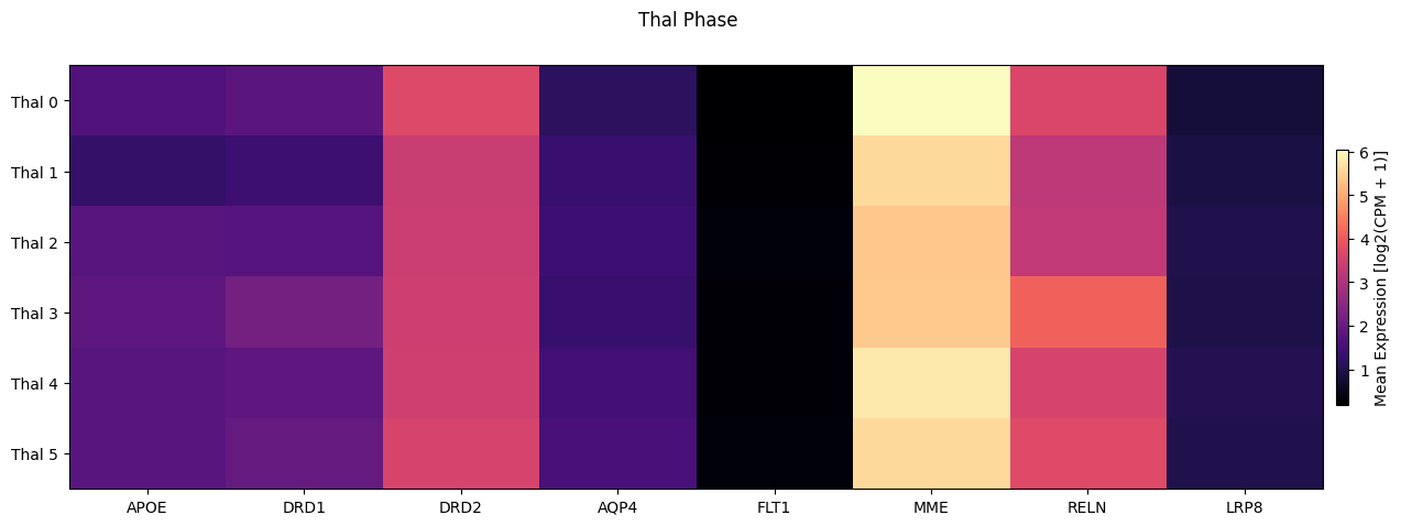
Finally we show the average expression in the heatmap vs one of the clinical markers. Here we use Thal Phase

fig, ax = plot_heatmap(
    df=cell_extended,
    gnames=gene_names,
    value='Thal',
    fig_width=15,
    fig_height=5,
    sort=True,
)
fig.suptitle('Thal Phase')
plt.show()

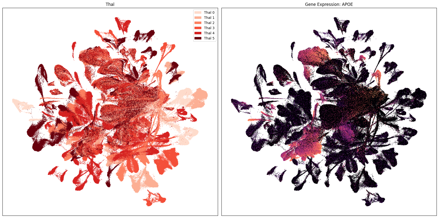
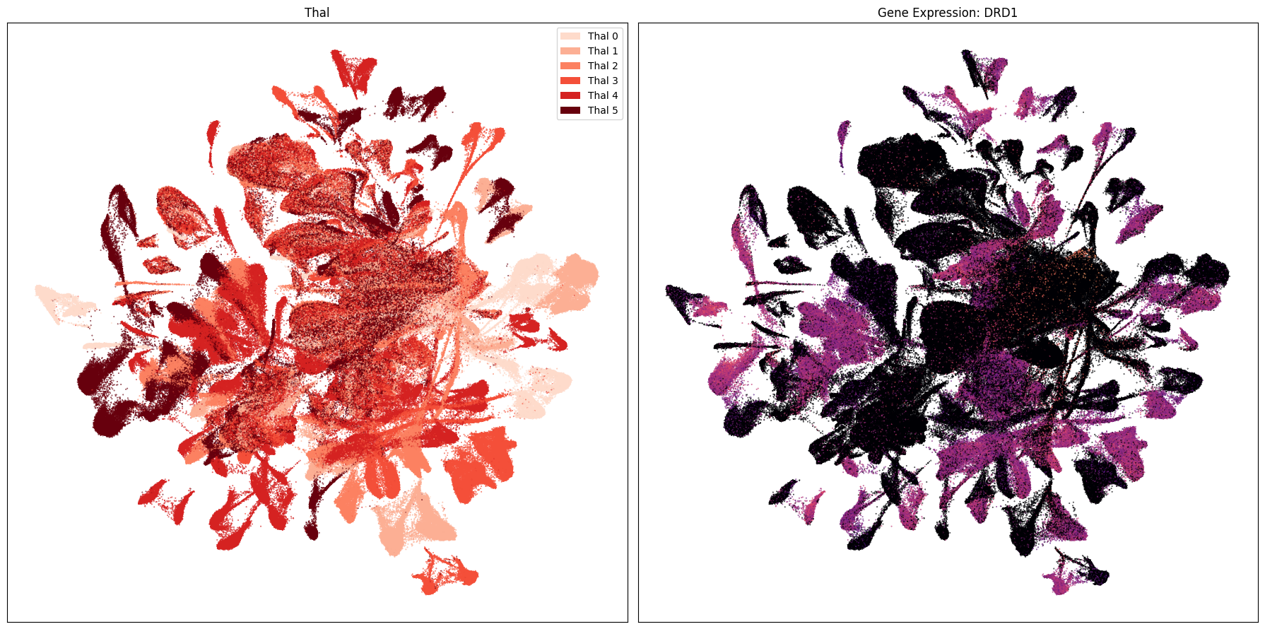
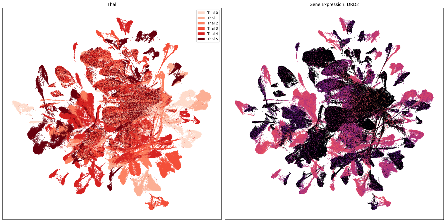
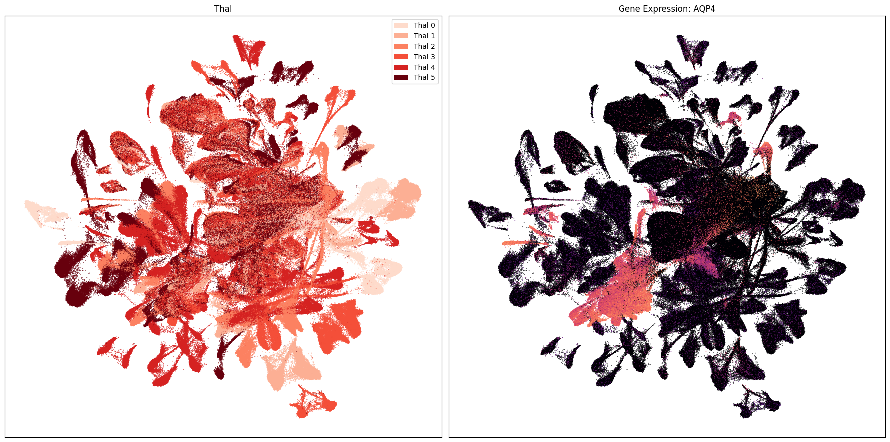
Expression in the UMAP

We load the UMAP coordinates for our cells and plot the expression in the UMAP for each of our selected genes. The UMAP is the same as the previous notebook.

cell_2d_embedding_coordinates = abc_cache.get_metadata_dataframe(
    directory='SEA-AD-CaH-taxonomy',
    file_name='cell_2d_embedding_coordinates'
).set_index('cell_label')
cell_2d_embedding_coordinates.head()

cell_2d_embedding_coordinates.csv: 100%|██████████| 41.1M/41.1M [00:04<00:00, 8.96MMB/s]  

	x	y
cell_label
AAACCCAAGAATCTAG-1336_B04	13.205919	4.357159
AAACCCAAGCACAAAT-1336_B04	13.403980	2.630821
AAACCCAAGGGACTGT-1336_B04	10.594164	1.961733
AAACCCACAATTTCCT-1336_B04	6.760588	0.988031
AAACCCACAGCAATTC-1336_B04	4.390634	3.214746

Join the coordinates into the cell metadata.

cell_extended = cell_extended.join(
    cell_2d_embedding_coordinates,
    how='inner'
).sample(frac=1)
cell_extended.head()

	cell_barcode	barcoded_cell_sample_label	library_label	alignment_job_id	doublet_score	umi_count	Used in analysis	donor_label	exp_component_name	feature_matrix_label	...	LRP8	MME	DRD1	RELN	DRD2	FLT1	AQP4	APOE	x	y
cell_label
CTGTTTAGTCAGGCAT-1520_B04	CTGTTTAGTCAGGCAT	1520_B04	L8XR_221201_02_A01	1233285482	0.04	1019.0	False	H21.33.001	CTGTTTAGTCAGGCAT-L8XR_221201_02_A01-1233285482	CaH-10X	...	0.0	0.000000	0.000000	0.000000	0.000000	0.000000	0.000000	0.000000	5.453426	-0.261755
CGTGCTTGTGTTAAAG-1190_C02	CGTGCTTGTGTTAAAG	1190_C02	L8HX_220407_03_C12	1173083446	0.00	3959.0	True	H21.33.039	CGTGCTTGTGTTAAAG-L8HX_220407_03_C12-1173083446	CaH-10X	...	0.0	0.000000	0.000000	8.983501	0.000000	0.000000	0.000000	0.000000	0.388968	1.094317
TTCCTAATCGCCGAGT-1235_B02	TTCCTAATCGCCGAGT	1235_B02	L8HX_220505_03_B07	1177380822	0.00	28241.0	True	H20.33.016	TTCCTAATCGCCGAGT-L8HX_220505_03_B07-1177380822	CaH-10X	...	0.0	8.151149	0.000000	5.186243	8.151149	0.000000	0.000000	0.000000	-4.895729	1.723459
ACGGTCGAGTCATGAA-1235_B01	ACGGTCGAGTCATGAA	1235_B01	L8HX_220505_03_E07	1177380819	0.00	56255.0	True	H20.33.001	ACGGTCGAGTCATGAA-L8HX_220505_03_E07-1177380819	CaH-10X	...	0.0	8.614991	6.750301	7.858544	0.000000	4.230833	4.230833	4.230833	0.216152	-8.710985
GTCCAGGGTATTGGTG-1467_C08	GTCCAGGGTATTGGTG	1467_C08	L8XR_221020_01_E05	1225051611	0.00	25463.0	True	H20.33.011	GTCCAGGGTATTGGTG-L8XR_221020_01_E05-1225051611	CaH-10X	...	0.0	9.105431	0.000000	0.000000	7.304608	0.000000	0.000000	0.000000	-8.339384	4.063814

5 rows × 115 columns

We use the same UMAP plotting convenience function as previously used in the SEA-AD CaH clustering and annotation tutorial.

def plot_umap(
    xx: np.ndarray,
    yy: np.ndarray,
    cc: np.ndarray = None,
    val: np.ndarray = None,
    fig_width: float = 8,
    fig_height: float = 8,
    cmap: Optional[plt.Colormap] = None,
    labels: np.ndarray = None,
    term_orders: np.ndarray = None,
    colorbar: bool = False,
    sizes: np.ndarray = None,
    fig: plt.Figure = None,
    ax: plt.Axes = None,
 ) -> Tuple[plt.Figure, plt.Axes]:
    """
    Plot a scatter plot of the UMAP coordinates.

    Parameters
    ----------
    xx : array-like
        x-coordinates of the points to plot.
    yy : array-like
        y-coordinates of the points to plot.
    cc : array-like, optional
        colors of the points to plot. If None, the points will be colored by the values in `val`.
    val : array-like, optional
        values of the points to plot. If None, the points will be colored by the values in `cc`.
    fig_width : float, optional
        width of the figure in inches. Default is 8.
    fig_height : float, optional
        height of the figure in inches. Default is 8.
    cmap : str, optional
        colormap to use for coloring the points. If None, the points will be colored by the values in `cc`.
    labels : array-like, optional
        labels for the points to plot. If None, no labels will be added to the plot.
    term_orders : array-like, optional
        order of the labels for the legend. If None, the labels will be ordered by their appearance in `labels`.
    colorbar : bool, optional
        whether to add a colorbar to the plot. Default is False.
    sizes : array-like, optional
        sizes of the points to plot. If None, all points will have the same size.
    fig : matplotlib.figure.Figure, optional
        figure to plot on. If None, a new figure will be created with 1 subplot.
    ax : matplotlib.axes.Axes, optional
        axes to plot on. If None, a new figure will be created with 1 subplot.
    """

    if sizes is None:
        sizes = 1
    if ax is None or fig is None:
        fig, ax = plt.subplots()
        fig.set_size_inches(fig_width, fig_height)

    if cmap is not None:
        scatt = ax.scatter(xx, yy, c=val, s=0.5, marker='.', cmap=cmap, alpha=sizes)
    elif cc is not None:
        scatt = ax.scatter(xx, yy, c=cc, s=0.5, marker='.', alpha=sizes)

    if labels is not None:
        from matplotlib.patches import Rectangle
        unique_label_colors = (labels + ',' + cc).unique()
        unique_labels = np.array([label_color.split(',')[0] for label_color in unique_label_colors])
        unique_colors = np.array([label_color.split(',')[1] for label_color in unique_label_colors])

        if term_orders is not None:
            unique_order = term_orders.unique()
            term_order = np.argsort(unique_order)
            unique_labels = unique_labels[term_order]
            unique_colors = unique_colors[term_order]
            
        rects = []
        for color in unique_colors:
            rects.append(Rectangle((0, 0), 1, 1, fc=color))

        legend = ax.legend(rects, unique_labels, loc=0)
        # ax.add_artist(legend)
    
    ax.set_xticks([])
    ax.set_yticks([])

    if colorbar:
        fig.colorbar(scatt, ax=ax)
    
    return fig, ax

Below we plot the genes in our set next to the UMAP colored by one of our features.

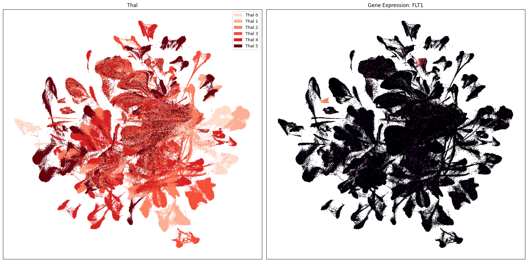
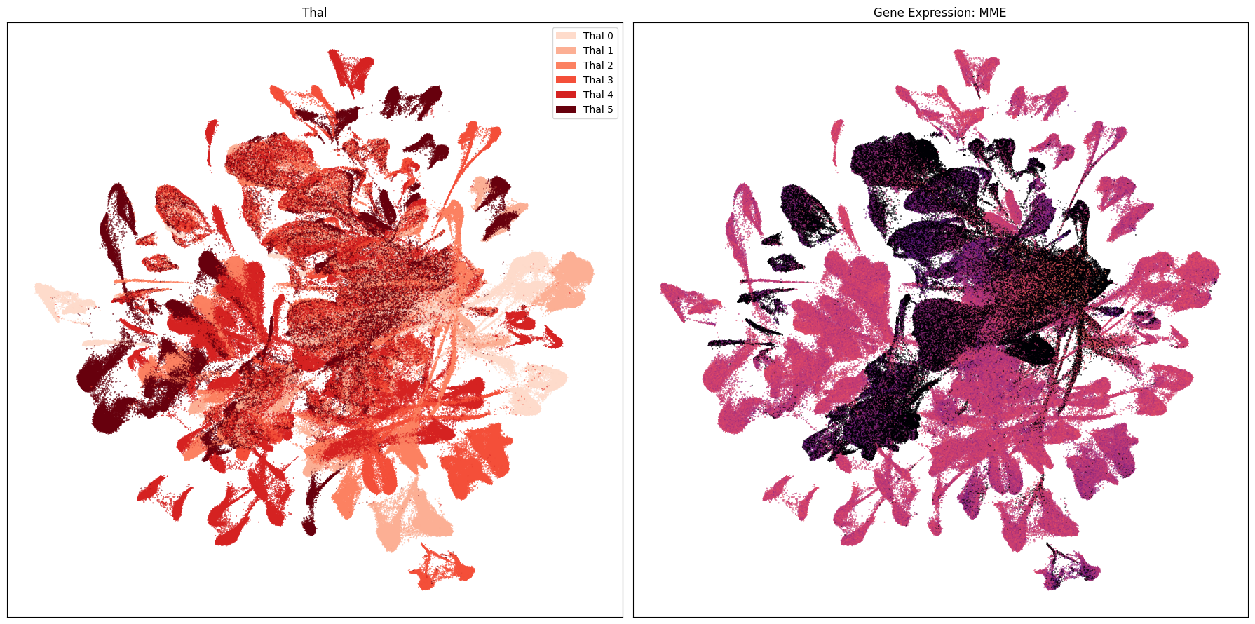
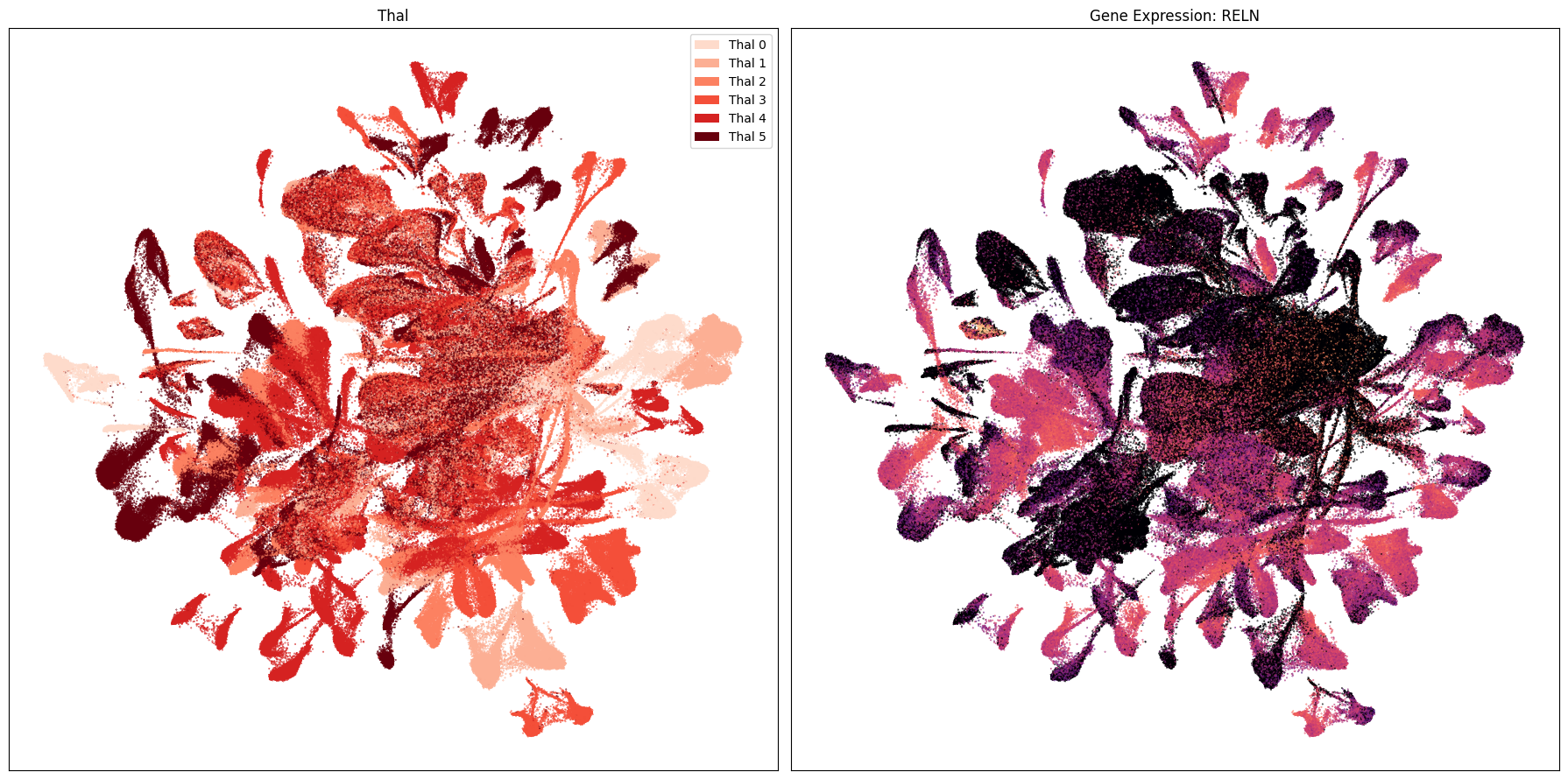
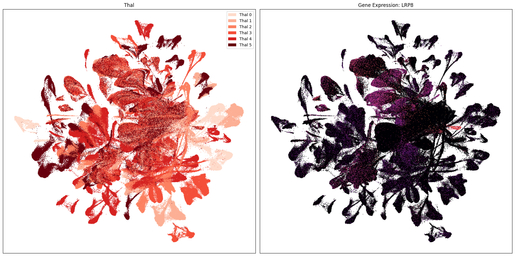
term_to_plot = 'Thal'

# Plot UMAPs for the first two genes in gene_names
for gene_name in gene_names:
    fig, ax = plt.subplots(1, 2)
    fig.set_size_inches(18, 9)
    ax = ax.flatten()
    plot_umap(
        cell_extended['x'],
        cell_extended['y'],
        cc=cell_extended[term_to_plot + '_color'],
        labels=cell_extended[term_to_plot],
        term_orders=cell_extended[term_to_plot + '_order'],
        fig=fig,
        ax=ax[0],
    )
    ax[0].set_title(term_to_plot)
    plot_umap(
        cell_extended['x'],
        cell_extended['y'],
        val=cell_extended[gene_name],
        cmap=plt.cm.magma,
        fig=fig,
        ax=ax[1],
        colorbar=False,
    )
    ax[1].set_title(f'Gene Expression: {gene_name}')
    plt.tight_layout()
    plt.show()

Also available is the SEA-AD CaH taxonomy notebook. You can also investigate the SEA-AD Multiregion data and taxonomy here.