Human-Mammalian Brain - Basal Ganglia Patchseq

The basal ganglia (BG) constitute a system of interconnected brain structures that play a crucial role in motor control, learning, behavior, and emotion. These structures are implicated in numerous disorders affecting human health, including Parkinson’s disease, Huntington’s disease, and substance abuse disorders. Despite their importance, little is known about the cellular-level functional properties of the BG in humans and translationally relevant primate species. To address this gap, we performed Patch-seq experiments – integrating patch clamp electrophysiology with single cell RNA-sequencing anchored in the high-resolution, cross-species HMBA consensus basal ganglia cell type taxonomy. This approach enables us to reveal the morpho-electric properties of transcriptomically-defined striatal cell types in primates. Following electrophysiological characterization, nuclei were aspirated for RNA sequencing (SMART-Seq v4), and transcriptomic profiles were mapped to the consensus taxonomy. Each sample was assigned spatial coordinates within an anatomical reference, and cells with high-quality fills and mappings were subsequently reconstructed to obtain morphological features. The data derive from macaque (Macaca mulatta and Macaca nemestrina) striatal tissue obtained through a Tissue Distribution Program. These data are directly comparable to mouse basal ganglia datasets collected using the same protocols.

Patch-seq samples were mapped to striatal neuronal types using the Hierarchical Approximate Nearest Neighbor (HANN) method implemented in the Allen Institute MapMyCells package, excluding non-neuronal types. After applying quality control to the mapping results, 717 macaque samples were retained. For more information on the taxonomy, please refer to the following webpage: Mammalian Basal Ganglia Consensus Cell Type Atlas. Additionally, you can see the associated notebooks linked at the end of this page.

In this notebook, we’ll look at gene expression for these 717 Macaque cells for different regions and taxonomy assignments. We’ll also look at the electrophysiology and morphology summary stats as a function of the taxonomy.

You need to be connected to the internet to run this notebook and have run through the getting started notebook.

from typing import List, Tuple, Optional

import pandas as pd
from pathlib import Path
import numpy as np
import matplotlib.pyplot as plt
import matplotlib as mpl

from abc_atlas_access.abc_atlas_cache.abc_project_cache import AbcProjectCache
from abc_atlas_access.abc_atlas_cache.anndata_utils import get_gene_data

We will interact with the data using the AbcProjectCache. This cache object tracks which data has been downloaded and serves the path to the requested data on disk. For metadata, the cache can also directly serve a up a Pandas DataFrame. See the getting_started notebook for more details on using the cache including installing the cache if it has not already been.

Change the download_base variable to where you would like to download the data in your system.

download_base = Path('../../data/abc_atlas')
abc_cache = AbcProjectCache.from_cache_dir(
    download_base,
)

abc_cache.current_manifest

'releases/20260228/manifest.json'

Cell metadata

Below we load the metadata associated with the individual patchseq cells and donor and library metadata. We join the donor and library data into the cell_metadata, this gives us e.g. donor_sex, donor_age information and region of interest labels from the library information.

macaque_cell_metadata = abc_cache.get_metadata_dataframe(
    directory='HMBA-Macaque-PatchSeq',
    file_name='cell_metadata',
    dtype={"cell_label": str}
).set_index('cell_label')

macaque_donor = abc_cache.get_metadata_dataframe(
    directory='HMBA-Macaque-PatchSeq',
    file_name='donor'
).set_index('donor_label')

macaque_library = abc_cache.get_metadata_dataframe(
    directory='HMBA-Macaque-PatchSeq',
    file_name='library'
).set_index('library_label')

macaque_cell_metadata = macaque_cell_metadata.join(macaque_donor, on='donor_label', rsuffix='_donor')
macaque_cell_metadata = macaque_cell_metadata.join(macaque_library, on='library_label', rsuffix='_library')
macaque_cell_metadata.head()

cell_metadata.csv: 100%|██████████| 109k/109k [00:00<00:00, 998kMB/s]
donor.csv: 100%|██████████| 6.56k/6.56k [00:00<00:00, 77.2kMB/s]
library.csv: 100%|██████████| 142k/142k [00:00<00:00, 919kMB/s]  

	library_label	library_aliquot_label	barcoded_cell_sample_label	donor_label	dataset_label	feature_matrix_label	alignment_id	donor_age_value	donor_age_unit	age_at_death_reference_point	...	library_aliquot_label_library	barcoded_cell_sample_label_library	barcoded_cell_sample_technique	amplified_cdna_label	tissue_sample_local_name	donor_label_library	region_of_interest_label	region_of_interest_id	library_aliquot_nhash_id	library_nhash_id
cell_label
QN22.26.002.14.05.04	L8S4_220222_04_H05	AB-S40302_S424_E1-50	P4S4_220131_155_A01	QN22.26.002	HMBA-Macaque-PatchSeq	HMBA-Macaque-PatchSeq-BG	1200710839	15	years	birth	...	AB-S40302_S424_E1-50	P4S4_220131_155_A01	PatchSeq-SmartSeq	A8S4_220215_06_H05	QN22.26.002.14.05	QN22.26.002	Ca	HOMBA:10334	LA-JEACHN795730XCYBFE242803	LI-JEACHN795730
QN22.26.002.14.05.05	L8S4_220222_04_A06	AB-S40302_S425_E1-50	P4S4_220131_156_A01	QN22.26.002	HMBA-Macaque-PatchSeq	HMBA-Macaque-PatchSeq-BG	1200710837	15	years	birth	...	AB-S40302_S425_E1-50	P4S4_220131_156_A01	PatchSeq-SmartSeq	A8S4_220215_06_A06	QN22.26.002.14.05	QN22.26.002	Ca	HOMBA:10334	LA-WCXYWT453000XCYBFE242803	LI-WCXYWT453000
QN22.26.002.14.05.06	L8S4_220222_04_B06	AB-S40302_S426_E1-50	P4S4_220131_157_A01	QN22.26.002	HMBA-Macaque-PatchSeq	HMBA-Macaque-PatchSeq-BG	1200710836	15	years	birth	...	AB-S40302_S426_E1-50	P4S4_220131_157_A01	PatchSeq-SmartSeq	A8S4_220215_06_B06	QN22.26.002.14.05	QN22.26.002	Ca	HOMBA:10334	LA-JMJMOH539975XCYBFE242803	LI-JMJMOH539975
QN22.26.002.14.05.08	L8S4_220222_04_C06	AB-S40302_S427_E1-50	P4S4_220131_158_A01	QN22.26.002	HMBA-Macaque-PatchSeq	HMBA-Macaque-PatchSeq-BG	1200710835	15	years	birth	...	AB-S40302_S427_E1-50	P4S4_220131_158_A01	PatchSeq-SmartSeq	A8S4_220215_06_C06	QN22.26.002.14.05	QN22.26.002	Ca	HOMBA:10334	LA-NJMQPI138328XCYBFE242803	LI-NJMQPI138328
QN22.26.002.14.05.09	L8S4_220222_04_D06	AB-S40302_S428_E1-50	P4S4_220131_159_A01	QN22.26.002	HMBA-Macaque-PatchSeq	HMBA-Macaque-PatchSeq-BG	1200710834	15	years	birth	...	AB-S40302_S428_E1-50	P4S4_220131_159_A01	PatchSeq-SmartSeq	A8S4_220215_06_D06	QN22.26.002.14.05	QN22.26.002	Ca	HOMBA:10334	LA-HIEYXR972206XCYBFE242803	LI-HIEYXR972206

5 rows × 27 columns

We load a value set table that defines colors for various features in the dataset as well as orders for those feature terms. We use these orders later in this notebook.

value_sets = abc_cache.get_metadata_dataframe(
    directory='HMBA-Macaque-PatchSeq',
    file_name='value_sets'
).set_index('label')
value_sets

value_sets.csv: 100%|██████████| 1.68k/1.68k [00:00<00:00, 26.1kMB/s]

	table	field	description	order	external_identifier	parent_label	color_hex_triplet
label
Female	donor	donor_sex	Female	1	NaN	NaN	#565353
Male	donor	donor_sex	Male	2	NaN	NaN	#ADC4C3
Human	donor	species_genus	Human	1	NCBITaxon:9605	NaN	#377eb8
Macaque	donor	species_genus	Macaque	2	NCBITaxon:9539	NaN	#4daf4a
Marmoset	donor	species_genus	Marmoset	3	NCBITaxon:9481	NaN	#FF5F5D
Squirrel monkey	donor	species_genus	Squirrel monkey	4	NCBITaxon:9520	NaN	#ffa300
Mouse	donor	species_genus	Mouse	5	NCBITaxon:10088	NaN	#c941a7
Homo sapiens	donor	species_scientific_name	Homo sapiens	1	NCBITaxon:9606	NaN	#377eb8
Macaca mulatta	donor	species_scientific_name	Macaca mulatta	2	NCBITaxon:9544	NaN	#4daf4a
Macaca nemestrina	donor	species_scientific_name	Macaca nemestrina	3	NCBITaxon:9545	NaN	#b2df8a
Callithrix jacchus	donor	species_scientific_name	Callithrix jacchus	4	NCBITaxon:9483	NaN	#FF5F5D
Saimiri sciureus	donor	species_scientific_name	Saimiri sciureus	5	NCBITaxon:9521	NaN	#FF5F5D
Mus musculus	donor	species_scientific_name	Mus musculus	6	NCBITaxon:10090	NaN	#ffa300
STR	library	region_of_interest_label	striatum (neostriatum)	1	HOMBA:10333	NaN	#048359
DS	library	region_of_interest_label	dorsal striatum (caudoputamen complex-CP, STRd)	2	HOMBA:AA30192	STR	#ff399a
Ca	library	region_of_interest_label	caudate nucleus (mediodorsal division of the CP)	3	HOMBA:10334	DS	#ff6b9a
Pu	library	region_of_interest_label	putamen (lateroventral division of the CP)	4	HOMBA:10338	DS	#9ba2ff
VS	library	region_of_interest_label	ventral striatum (STRv)	5	HOMBA:AA30195	STR	#ffe119
NAC	library	region_of_interest_label	nucleus accumbens	6	HOMBA:10339	VS	#c29515
ic	library	region_of_interest_label	internal capsule	7	HOMBA:10581	NaN	#ffd7b4

We define a convenience function to add colors for the various values in the data (e.g. unique region of interest or donor sex values).

def extract_value_set(cell_metadata_df: pd.DataFrame, input_value_set: pd.DataFrame, input_value_set_label: str):
    """Add color and order columns to the cell metadata dataframe based on the input
    value set.

    Columns are added as {input_value_set_label}_color and {input_value_set_label}_order.

    Parameters
    ----------
    cell_metadata_df : pd.DataFrame
        DataFrame containing cell metadata.
    input_value_set : pd.DataFrame
        DataFrame containing the value set information.
    input_value_set_label : str
        The column name to extract color and order information for. The information will then be added to
        the cell metadata.
    """
    cell_metadata_df[f'{input_value_set_label}_color'] = input_value_set[
        input_value_set['field'] == input_value_set_label
    ].loc[cell_metadata_df[input_value_set_label]]['color_hex_triplet'].values
    cell_metadata_df[f'{input_value_set_label}_order'] = input_value_set[
        input_value_set['field'] == input_value_set_label
    ].loc[cell_metadata_df[input_value_set_label]]['order'].values

Use our function to add the relevant color and order columns to our cell_metadata table.

# Add region of interest color and order
extract_value_set(macaque_cell_metadata, value_sets, 'region_of_interest_label')

Gene expression data

Now we extract expression for specific genes from the h5ad files and pair it with our gene metadata. In general, we can use the function get_gene_data to extract the expression of specific genes for all the cells in a given dataset or a subset of cells. For more details on using this convenience function, see the Accessing 10x RNA-seq gene expression data tutorial notebook.

For this tutorial we will use precomputed tables of the expression for specific genes to compare expression by spatial location or by transcriptomic group.

To use the gene expression data, we first load the set of genes for the patch-seq data.

macaque_genes = abc_cache.get_metadata_dataframe(
    directory='HMBA-Macaque-PatchSeq',
    file_name='gene',
).set_index('gene_identifier')
macaque_genes.head()

gene.csv: 100%|██████████| 3.33M/3.33M [00:00<00:00, 9.36MMB/s]

	gene_symbol	description	gene_id	molecular_type	synonym
gene_identifier
NCBIGene:712737	A1BG	alpha-1-B glycoprotein	712737	protein_coding	[]
NCBIGene:703806	A1CF	APOBEC1 complementation factor	703806	protein_coding	[]
NCBIGene:716616	A2ML1	alpha-2-macroglobulin like 1	716616	protein_coding	[]
NCBIGene:711045	A3GALT2	alpha 1,3-galactosyltransferase 2	711045	protein_coding	[]
NCBIGene:710998	A4GALT	alpha 1,4-galactosyltransferase	710998	protein_coding	[]

Below we list the genes we will use in this notebook and the example method used to load the expression for these specific genes from the h5ad file. More details on how to extract specific genes from the data see our accessing gene expression data tutorial

gene_names = ["WFS1", "CNR1", "CHRM3", "MYO16", "PTHLH", "DRD1", "DRD2", "TAC3", "SST"] 

macaque_gene_data = get_gene_data(
    abc_atlas_cache=abc_cache,
    all_cells=macaque_cell_metadata,
    all_genes=macaque_genes,
    selected_genes=gene_names,
    data_type='log2'
)
macaque_gene_data.head()

loading file: HMBA-Macaque-PatchSeq-BG

HMBA-Macaque-PatchSeq-BG-log2.h5ad: 100%|██████████| 63.8M/63.8M [00:02<00:00, 23.9MMB/s]  

 - time taken:  0.115348
total time taken: 0.905653
	total cells: 717 processed cells: 717

gene_symbol	CHRM3	CNR1	DRD1	DRD2	MYO16	PTHLH	SST	TAC3	WFS1
cell_label
QN22.26.002.14.05.04	10.811937	0.000000	0.000000	8.153246	4.933148	3.680369	6.044661	0.0	5.300721
QN22.26.002.14.05.05	2.088328	5.323032	6.759345	0.000000	0.000000	4.358629	0.000000	0.0	0.000000
QN22.26.002.14.05.06	7.193662	0.000000	0.000000	7.467582	4.027162	0.000000	0.000000	0.0	6.536435
QN22.26.002.14.05.08	7.406147	0.000000	0.000000	7.258967	6.859893	2.354068	0.000000	0.0	3.205592
QN22.26.002.14.05.09	9.808509	0.000000	8.067217	0.000000	0.000000	0.000000	0.000000	0.0	6.322538

Now that we’ve loaded our expression matrix tables, indexed by cell_label, we can merge them into our cell metadata tables.

macaque_cell_metadata_with_genes = macaque_cell_metadata.join(macaque_gene_data, on='cell_label')

Plotting heatmap expression data

We define a helper functions aggregate_by_metadata to compute the average expression for a given category. Note that this is a simple wrapper of the Pandas GroupBy functionality. Other summary statistics beyond just the mean are listed here: https://pandas.pydata.org/docs/reference/groupby.html#dataframegroupby-computations-descriptive-stats

We also define a function to plot the resultant averaged data in a heatmap.

def aggregate_by_metadata(df: pd.DataFrame, gnames: List[str], value: str, sort: bool = False) -> pd.DataFrame:
    """Aggregate gene expression data by metadata.

    Parameters
    ----------
    df: pandas.DataFrame
        DataFrame containing gene expression and metadata.
    gnames: List[str]
        List of gene names to aggregate.
    value: str
        Metadata column to group by.
    sort: bool
        If True, sort the output by the first gene in gnames.

    Returns
    -------
    pandas.DataFrame
        DataFrame with aggregated gene expression values.
    """
    grouped = df.groupby(value)[gnames].mean()
    if sort:
        grouped = grouped.sort_values(by=gnames[0], ascending=False)
    if f'{value}_order' in df.columns:
        grouped = grouped.loc[df[value].unique()[np.argsort(df[value + '_order'].unique())]]
    return grouped


def plot_heatmap(
        df: pd.DataFrame,
        fig_width: int = 8,
        fig_height: int = 4,
        cmap: mpl.colormaps = plt.cm.magma,
        vmin: Optional[float] = None,
        vmax: Optional[float] = None,
        unit: str = '[log2(CPM + 1)]'
    ) -> Tuple[plt.Figure, plt.Axes]:
    """Plot a heatmap from a DataFrame.

    Parameters
    ----------
    df: pandas.DataFrame
        DataFrame to plot as a heatmap.
    fig_width: int
        Width of the figure (inches).
    fig_height: int
        Height of the figure (inches).
    cmap: matplotlib.colors.Colormap
        Colormap to use for the heatmap.

    Returns
    -------
    fig: matplotlib.pyplot.Figure
        Figure object containing the heatmap.
    ax: matplotlib.pyplot.Axes
        Axes object containing the heatmap.
    """

    arr = df.to_numpy().astype('float')

    if vmin is None:
        vmin = arr.min()
    if vmax is None:
        vmax = arr.max()
    norm = mpl.colors.Normalize(vmin=vmin, vmax=vmax)
    sm = plt.cm.ScalarMappable(cmap=cmap, norm=norm)
    cmap = sm.get_cmap()

    fig, ax = plt.subplots()
    fig.set_size_inches(fig_width, fig_height)

    ax.imshow(arr, cmap=cmap, aspect='auto', vmin=vmin, vmax=vmax)
    xlabs = df.columns.values
    ylabs = df.index.values

    ax.set_xticks(range(len(xlabs)))
    ax.set_xticklabels(xlabs)

    ax.set_yticks(range(len(ylabs)))
    ax.set_yticklabels(ylabs)

    cbar = fig.colorbar(sm, ax=ax, orientation='vertical', fraction=0.1, pad=0.01)
    cbar.set_label(unit)

    return fig, ax

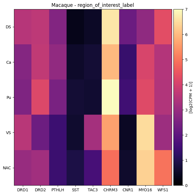
Visualize gene expression for selected genes by ROI

We plot the gene expression as a heat map showing the average expression as a function of region of interest (ROI) label. The full names for the region of interest acronyms can be found in the values_sets table we loaded earlier. Note that samples that were not precisely pinned anatomically were assigned to dorsal or ventral striatum based on the patch-clamp experimentalist’s original notes.

macaque_gene_names = ['DRD1', 'DRD2', 'PTHLH', 'SST', 'TAC3', 'CHRM3', 'CNR1', 'MYO16', 'WFS1']

feature_name = "region_of_interest_label"
agg = aggregate_by_metadata(macaque_cell_metadata_with_genes, macaque_gene_names, feature_name)
# We drop ic here as it has a very small number or cells.
plot_heatmap(agg.drop('ic'), 8, 8, vmin=0, vmax=7) # vmin and vmax set based on observed expression ranges
plt.title(f'Macaque - {feature_name}')
plt.show()

Taxonomy mapping

Finally, let’s load the taxonomy information so that we can plot gene expression versus various taxons in a heatmap for each species. Below, we load and merge all the information we need to plot cell colors and taxonomy as done in the previous HMBA tutorial.

cluster = abc_cache.get_metadata_dataframe(
    directory='HMBA-BG-taxonomy-CCN20250428',
    file_name='cluster',
    dtype={'number_of_cells': 'Int64'}
).rename(columns={'label': 'cluster_annotation_term_label'}).set_index('cluster_annotation_term_label')
cluster_annotation_term_set = abc_cache.get_metadata_dataframe(
    directory='HMBA-BG-taxonomy-CCN20250428',
    file_name='cluster_annotation_term_set'
).rename(columns={'label': 'cluster_annotation_term_label'})

cluster_annotation_term = abc_cache.get_metadata_dataframe(
    directory='HMBA-BG-taxonomy-CCN20250428',
    file_name='cluster_annotation_term',
).rename(columns={'label': 'cluster_annotation_term_label'}).set_index('cluster_annotation_term_label')

cluster_to_cluster_annotation_membership = abc_cache.get_metadata_dataframe(
    directory='HMBA-BG-taxonomy-CCN20250428',
    file_name='cluster_to_cluster_annotation_membership',
).set_index('cluster_annotation_term_label')
membership_with_cluster_info = cluster_to_cluster_annotation_membership.join(
    cluster.reset_index().set_index('cluster_alias')[['number_of_cells']],
    on='cluster_alias'
)
membership_with_cluster_info = membership_with_cluster_info.join(cluster_annotation_term, rsuffix='_anno_term').reset_index()
membership_groupby = membership_with_cluster_info.groupby(
    ['cluster_alias', 'cluster_annotation_term_set_name']
)

cluster_annotation_term_set = abc_cache.get_metadata_dataframe(
    directory='HMBA-BG-taxonomy-CCN20250428',
    file_name='cluster_annotation_term_set'
).rename(columns={'label': 'cluster_annotation_term_label'})

# term_sets = abc_cache.get_metadata_dataframe(directory='WHB-taxonomy', file_name='cluster_annotation_term_set').set_index('label')
cluster_details = membership_groupby['cluster_annotation_term_name'].first().unstack()
cluster_order = membership_groupby['term_order'].first().unstack()
cluster_order.sort_values(['Neighborhood', 'Class', 'Subclass', 'Group', 'Cluster'], inplace=True)
cluster_order.rename(
    columns={'Neighborhood': 'Neighborhood_order',
             'Class': 'Class_order',
             'Subclass': 'Subclass_order',
             'Group': 'Group_order',
             'Cluster': 'Cluster_order'},
    inplace=True
)

cluster_colors = membership_groupby['color_hex_triplet'].first().unstack()
cluster_colors = cluster_colors[cluster_annotation_term_set['name']]
cluster_colors.sort_values(
    ['Neighborhood', 'Class', 'Subclass', 'Group', 'Cluster'],
    inplace=True
)

The macaque patch-seq gene expression has been mapped to the HMBA-BG taxonomy using MapMyCells, excluding non-neuronal nodes. We load this table below. A more lightweight version of this table with only mappings between cells to cluster_alias. The table is named cell_to_cluster_membership.

Below we load the complete MMC results with probabilities and correlation coefficients for all assignments at all levels.

macaque_mmc = abc_cache.get_metadata_dataframe(
    directory='HMBA-Macaque-PatchSeq',
    file_name='mmc_results',
).set_index('cell_label')
macaque_mmc.head()

mmc_results.csv: 100%|██████████| 201k/201k [00:00<00:00, 1.42MMB/s] 

	Neighborhood_label	Neighborhood_name	Neighborhood_bootstrapping_probability	Neighborhood_aggregate_probability	Neighborhood_correlation_coefficient	Class_label	Class_name	Class_bootstrapping_probability	Class_aggregate_probability	Class_correlation_coefficient	...	Group_label	Group_name	Group_bootstrapping_probability	Group_aggregate_probability	Group_correlation_coefficient	Cluster_label	cluster_alias	Cluster_bootstrapping_probability	Cluster_aggregate_probability	Cluster_correlation_coefficient
cell_label
QN22.26.002.14.05.04	CS20250428_NEIGH_0002	Subpallium GABA	1.0	1.0	0.7190	CS20250428_CLASS_0003	CN LGE GABA	1.0	1.0	0.7093	...	CS20250428_GROUP_0054	STRd D2 Striosome MSN	1.00	1.00	0.5715	CS20250428_CLUST_0986	Macaque-429	1.00	1.0000	0.5615
QN22.26.002.14.05.05	CS20250428_NEIGH_0002	Subpallium GABA	1.0	1.0	0.7634	CS20250428_CLASS_0003	CN LGE GABA	1.0	1.0	0.7466	...	CS20250428_GROUP_0049	STRd D1 Matrix MSN	1.00	1.00	0.6477	CS20250428_CLUST_0949	Macaque-467	0.99	0.9900	0.5517
QN22.26.002.14.05.06	CS20250428_NEIGH_0002	Subpallium GABA	1.0	1.0	0.6603	CS20250428_CLASS_0003	CN LGE GABA	1.0	1.0	0.6376	...	CS20250428_GROUP_0054	STRd D2 Striosome MSN	1.00	1.00	0.4564	CS20250428_CLUST_0986	Macaque-429	0.62	0.6200	0.4341
QN22.26.002.14.05.08	CS20250428_NEIGH_0002	Subpallium GABA	1.0	1.0	0.6162	CS20250428_CLASS_0003	CN LGE GABA	1.0	1.0	0.5980	...	CS20250428_GROUP_0052	STRd D2 Matrix MSN	0.88	0.88	0.4317	CS20250428_CLUST_0973	Macaque-465	1.00	0.8800	0.4515
QN22.26.002.14.05.09	CS20250428_NEIGH_0002	Subpallium GABA	1.0	1.0	0.6987	CS20250428_CLASS_0003	CN LGE GABA	1.0	1.0	0.6847	...	CS20250428_GROUP_0049	STRd D1 Matrix MSN	0.99	0.99	0.5025	CS20250428_CLUST_0949	Macaque-467	0.57	0.5643	0.3415

5 rows × 25 columns

macaque_cell_metadata_with_genes = macaque_cell_metadata_with_genes.join(macaque_mmc)
macaque_cell_metadata_with_genes = macaque_cell_metadata_with_genes.join(cluster_details, on='cluster_alias')
macaque_cell_metadata_with_genes = macaque_cell_metadata_with_genes.join(cluster_colors, on='cluster_alias', rsuffix='_color')
macaque_cell_metadata_with_genes = macaque_cell_metadata_with_genes.join(cluster_order, on='cluster_alias')

macaque_cell_metadata_with_genes.head()

	library_label	library_aliquot_label	barcoded_cell_sample_label	donor_label	dataset_label	feature_matrix_label	alignment_id	donor_age_value	donor_age_unit	age_at_death_reference_point	...	Neighborhood_color	Class_color	Subclass_color	Group_color	Cluster_color	Class_order	Cluster_order	Group_order	Neighborhood_order	Subclass_order
cell_label
QN22.26.002.14.05.04	L8S4_220222_04_H05	AB-S40302_S424_E1-50	P4S4_220131_155_A01	QN22.26.002	HMBA-Macaque-PatchSeq	HMBA-Macaque-PatchSeq-BG	1200710839	15	years	birth	...	#19613b	#d0b83c	#253c8c	#ff9896	#561430	10	1290	55	3	32
QN22.26.002.14.05.05	L8S4_220222_04_A06	AB-S40302_S425_E1-50	P4S4_220131_156_A01	QN22.26.002	HMBA-Macaque-PatchSeq	HMBA-Macaque-PatchSeq-BG	1200710837	15	years	birth	...	#19613b	#d0b83c	#1655f2	#1f77b4	#b83642	10	1059	50	3	31
QN22.26.002.14.05.06	L8S4_220222_04_B06	AB-S40302_S426_E1-50	P4S4_220131_157_A01	QN22.26.002	HMBA-Macaque-PatchSeq	HMBA-Macaque-PatchSeq-BG	1200710836	15	years	birth	...	#19613b	#d0b83c	#253c8c	#ff9896	#561430	10	1290	55	3	32
QN22.26.002.14.05.08	L8S4_220222_04_C06	AB-S40302_S427_E1-50	P4S4_220131_158_A01	QN22.26.002	HMBA-Macaque-PatchSeq	HMBA-Macaque-PatchSeq-BG	1200710835	15	years	birth	...	#19613b	#d0b83c	#253c8c	#aec7e8	#d71b39	10	1194	53	3	32
QN22.26.002.14.05.09	L8S4_220222_04_D06	AB-S40302_S428_E1-50	P4S4_220131_159_A01	QN22.26.002	HMBA-Macaque-PatchSeq	HMBA-Macaque-PatchSeq-BG	1200710834	15	years	birth	...	#19613b	#d0b83c	#1655f2	#1f77b4	#b83642	10	1059	50	3	31

5 rows × 78 columns

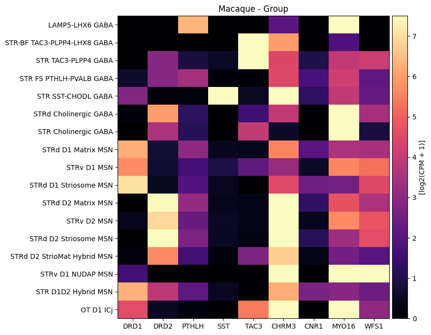
Visualize gene expression for selected genes by the HMBA-BG taxonomy

Below we plot the gene expression for the cells as a function the Group level in the taxonomy they were associated with. We plot the MSNs cell-types only. We’ll also use a subset of the genes we extracted from the gene expression matrix.

macaque_gene_names = ['DRD1', 'DRD2', 'PTHLH', 'SST', 'TAC3', 'CHRM3', 'CNR1', 'MYO16', 'WFS1']

feature_name = "Group"
agg = aggregate_by_metadata(
    macaque_cell_metadata_with_genes,
    macaque_gene_names,
    feature_name
)


plot_heatmap(agg, 8, 8, vmin=0, vmax=7.5)
plt.title(f'Macaque - {feature_name}')
plt.show()

Other Features

In addition to gene expression, we also look at electrophysiology and morphology features.

Electrophysiological features

The electrophysiological features are across 4 tables: ap_features, chirp_features, cross_sweep_long_square_features, and sweep_features. In the below example, we load the ap_features table and merge it into our cell_metadata table.

A full list of the electrophysiological features with some short descriptions can be downloaded here

ap_features = abc_cache.get_metadata_dataframe(
    directory='HMBA-Macaque-PatchSeq', file_name='ap_features'
).set_index('cell_label')

# most cells have no measurement for these features so we filter those with values just to see what the data looks like. 
ap_features[pd.notna(ap_features['adp_v_last_rheo'])].head()

ap_features.csv: 100%|██████████| 496k/496k [00:00<00:00, 3.00MMB/s] 

	adp_v_last_rheo	ahp_delay_5spike	ahp_delay_hero	ahp_delay_ratio_5spike	ahp_delay_ratio_hero	downstroke_adapt_ratio	downstroke_hero	downstroke_ramp	downstroke_rheo	downstroke_short_square	...	width_adapt_ratio	width_hero	width_ramp	width_rheo	width_rheo_ms	width_short_square	width_suprathresh_hero	width_suprathresh_ramp	width_suprathresh_rheo	width_suprathresh_short_square
cell_label
Q21.26.003.12.03.01	-55.000004	0.021870	0.000980	0.191146	0.034789	0.879896	-267.810016	NaN	-256.109021	-277.295319	...	1.090909	0.000375	NaN	0.000385	0.385	0.000370	0.000345	NaN	0.000355	0.000335
Q21.26.006.14.01.04	-50.093750	0.043635	0.043635	0.237018	0.237018	0.879694	-87.819662	NaN	-88.143416	-99.554269	...	1.086124	0.001045	NaN	0.001055	1.055	0.000935	0.000945	NaN	0.000955	0.000850
Q21.26.009.12.01.03	-51.000004	0.155950	0.001390	0.483124	0.066763	0.900912	-179.379158	NaN	-169.956722	-191.220558	...	1.070707	0.000475	NaN	0.000485	0.485	0.000460	0.000430	NaN	0.000455	0.000415
Q21.26.009.12.02.03	-61.062504	0.030185	0.026850	0.120473	0.188131	0.789810	-72.779128	NaN	-69.267846	-80.596543	...	1.152610	0.001270	NaN	0.001305	1.305	0.001220	0.001175	NaN	0.001185	0.001125
Q21.26.009.12.01.04	-52.812500	0.037275	0.026275	0.250311	0.255842	0.982069	-73.422130	NaN	-71.413402	-79.772097	...	1.101770	0.001120	NaN	0.001140	1.140	0.001085	0.001045	NaN	0.001050	0.000990

5 rows × 57 columns

macaque_cell_metadata_with_genes = macaque_cell_metadata_with_genes.join(ap_features)

Below, we create a function to create a box plot for a given feature by e.g. a taxonomy level, ROI structure, etc.

def plot_boxplot_by_column(
        dataframe, col_name, value_col
    ):
    """
    Plots a boxplot of the specified value column grouped by the specified column.

    Parameters
    ----------
    dataframe : pd.DataFrame
        The input dataframe containing the data to plot.
    col_name : str
        The name of the column to group by.
    value_col : str
        The name of the column containing the values to plot.
    """
    box_values = {}
    for group in dataframe[col_name].unique()[
            np.argsort(dataframe[f"{col_name}_order"].unique()) # Order by the specified order column
    ]:
        col_values = dataframe.loc[dataframe[col_name] == group, value_col]
        if pd.notna(col_values).sum() > 0:
            box_values[group] = col_values[~col_values.isna()].values # Use non-NA values for the boxplot

    plt.boxplot(
        box_values.values()
    )
    plt.xticks(
        ticks=np.arange(1, len(box_values) + 1),
        labels=box_values.keys(),
        rotation=90
    )
    plt.ylabel(value_col)
    plt.title(f'{value_col} by {col_name}')
    plt.show()

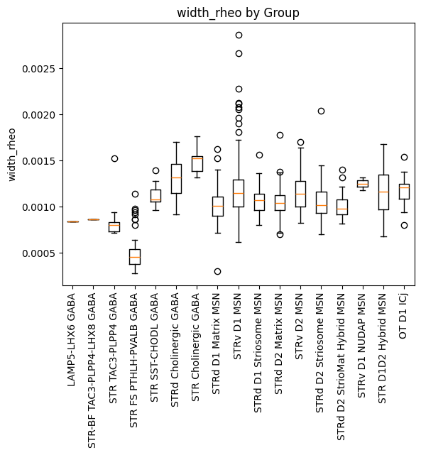
We’ll plot the ephys feature, width_rheo in a boxplot against the Groups in this dataset.

plot_boxplot_by_column(dataframe=macaque_cell_metadata_with_genes, col_name='Group', value_col='width_rheo')

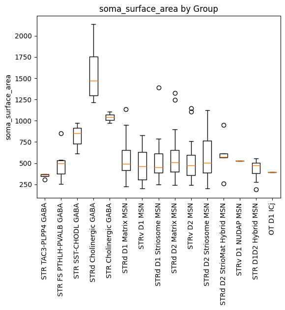
Morphological Features

We now load our morphological features and merge them into the cell metadata. A full list of the morphological features with short descriptions can be downloaded here.

morphology_features = abc_cache.get_metadata_dataframe(
    directory='HMBA-Macaque-PatchSeq', file_name='morphology_features'
).set_index('cell_label')
morphology_features.head()

morphology_features.csv: 100%|██████████| 97.4k/97.4k [00:00<00:00, 642kMB/s] 

	23_Sholl_PC0	23_Sholl_PC1	2_Sholl_PC0	2_Sholl_PC1	3_Sholl_PC0	3_Sholl_PC1	axon_bias_dorsal	axon_bias_medial	axon_exit_distance	axon_exit_theta_coronal	...	basal_dendrite_mean_diameter	basal_dendrite_num_branches	basal_dendrite_soma_percentile_dorsal	basal_dendrite_soma_percentile_medial	basal_dendrite_stem_exit_MedialLateral	basal_dendrite_stem_exit_dorsal	basal_dendrite_stem_exit_ventral	basal_dendrite_total_length	basal_dendrite_total_surface_area	soma_surface_area
cell_label
Q19.26.014.11.04.01	NaN	NaN	NaN	NaN	NaN	NaN	NaN	NaN	NaN	NaN	...	NaN	NaN	NaN	NaN	NaN	NaN	NaN	NaN	NaN	NaN
Q19.26.014.11.01.01	NaN	NaN	NaN	NaN	NaN	NaN	NaN	NaN	NaN	NaN	...	NaN	NaN	NaN	NaN	NaN	NaN	NaN	NaN	NaN	NaN
Q19.26.014.11.01.04	NaN	NaN	NaN	NaN	168.820400	29.150249	NaN	NaN	NaN	0.667150	...	0.573221	56.0	0.468694	0.334369	0.5	0.125	0.375	5241.027500	9442.031612	548.486434
Q19.26.014.11.01.05	NaN	NaN	NaN	NaN	282.741349	-36.067186	NaN	NaN	NaN	0.875211	...	0.565709	69.0	0.489853	0.428372	0.4	0.200	0.400	5909.886270	10526.672804	359.438955
Q19.26.014.11.05.01	NaN	NaN	NaN	NaN	276.829831	-84.814559	NaN	NaN	NaN	0.447964	...	0.609324	77.0	0.576005	0.407282	0.8	0.200	0.000	5946.308781	11421.095519	502.026310

5 rows × 39 columns

macaque_cell_metadata_with_genes = macaque_cell_metadata_with_genes.join(morphology_features)

Finally, we plot the soma surface area feature against the taxonomy Group.

plot_boxplot_by_column(dataframe=macaque_cell_metadata_with_genes, col_name='Group', value_col='soma_surface_area')

To learn more about the spatial transcriptomic data see the HMBA-BG Spatial Slabs and Taxonomy notebook.

To learn more about the taxonomy used in this notebook and the data it is derived from, see the HMBA-BG Clustering Analysis and Taxonomy notebook.