Human-Mammalian Brain - Basal Ganglia spatial transcriptomic slab coordinates and annotation

The basal ganglia are a set of subcortical structures critical for motor control, particularly in the context of action selection, motor learning and emotional state, whose coarse functional organization is well-described in the literature. Although single-cell RNA-Seq studies have greatly enhanced our understanding of cellular diversity in the brain, the exact spatial distribution of cell types within the brain has been difficult to determine. Using spatial transcriptomics platforms such as MERSCOPE or Xenium enables spatial profiling of hundreds of genes for each cell, enabling mapping of the cells to the consensus basal ganglia cell type taxonomy.

In this notebook, we walk through the data available in this release and show how they are joined together to enable analyses at the cell level.

You need to be connected to the internet to run this notebook and have run through the getting started notebook.

import json
import geojson
from typing import List, Tuple, Optional

import pandas as pd
from pathlib import Path
import numpy as np
import matplotlib.pyplot as plt

from abc_atlas_access.abc_atlas_cache.abc_project_cache import AbcProjectCache

We will interact with the data using the AbcProjectCache. This cache object tracks which data has been downloaded and serves the path to the requested data on disk. For metadata, the cache can also directly serve up a Pandas DataFrame. See the getting_started notebook for more details on using the cache including installing it if it has not already been.

Change the download_base variable to where you would like to download the data in your system.

download_base = Path('../../data/abc_atlas')
abc_cache = AbcProjectCache.from_cache_dir(
    download_base,
)

abc_cache.current_manifest

'releases/20250930/manifest.json'

Data Overview

Below we list the available metadata and expression matrix files available for each species.

The various species in this dataset are divided up by their donor_id and transcriptomic platform. MERSCOPE for Human and Macaque, Xenium for Marmoset.

The mapping between donor to species is:

• Human: H22.30.001

• Macaque: QM23.50.001

• Marmoset: CJ23.56.004

for dataset_name in ['HMBA-MERSCOPE-H22.30.001-BG', 'HMBA-MERSCOPE-QM23.50.001-BG', 'HMBA-Xenium-CJ23.56.004-BG']:
    print(f"Dataset: {dataset_name}")
    metadata_files = abc_cache.list_metadata_files(dataset_name)
    print(f"Metadata files: {metadata_files}")
    expression_matrix_files = abc_cache.list_expression_matrix_files(dataset_name)
    print(f"Expression matrix files: {expression_matrix_files}\n")

Dataset: HMBA-MERSCOPE-H22.30.001-BG
Metadata files: ['cell_anatomical_annotations', 'cell_metadata', 'cell_supplemental_metadata', 'cell_to_cluster_membership', 'donor', 'example_gene_expression', 'gene', 'mmc_results', 'slab_plane_coordinates', 'specimen_metadata', 'value_sets', 'visualization']
Expression matrix files: ['MERSCOPE-H22.30.001-BG/log2', 'MERSCOPE-H22.30.001-BG/raw']

Dataset: HMBA-MERSCOPE-QM23.50.001-BG
Metadata files: ['cell_anatomical_annotations', 'cell_metadata', 'cell_supplemental_metadata', 'cell_to_cluster_membership', 'donor', 'example_gene_expression', 'gene', 'mmc_results', 'slab_plane_coordinates', 'specimen_metadata', 'value_sets', 'visualization']
Expression matrix files: ['MERSCOPE-QM23.50.001-BG/log2', 'MERSCOPE-QM23.50.001-BG/raw']

Dataset: HMBA-Xenium-CJ23.56.004-BG
Metadata files: ['cell_anatomical_annotations', 'cell_metadata', 'cell_supplemental_metadata', 'cell_to_cluster_membership', 'donor', 'example_gene_expression', 'gene', 'mmc_results', 'slab_plane_coordinates', 'specimen_metadata', 'value_sets', 'visualization']
Expression matrix files: ['Xenium-CJ23.56.004-BG/log2', 'Xenium-CJ23.56.004-BG/raw']

Cell metadata

Each species in the HMBA spatial dataset has it’s own h5ad files and associated cell metadata tables. We load each of these in turn starting from Human to Macaque to Marmoset. These metadata contain the basic identifiers for each cell and forms the basis by which we will join all other cell level and associated data. Below we load the cell metadata for each species.

Load the Human cells.

human_cell_metadata = abc_cache.get_metadata_dataframe(
    directory='HMBA-MERSCOPE-H22.30.001-BG',
    file_name='cell_metadata',
    dtype={"cell_label": str}
).set_index('cell_label')
human_cell_metadata.head()

cell_metadata.csv: 100%|██████████| 996M/996M [00:28<00:00, 35.1MMB/s]    

	brain_section_label	brain_section_barcode	segmentation_job_id	x_experiment	y_experiment	qc_pass	dataset_label	feature_matrix_label	abc_sample_id
cell_label
1324989690_1-20250227	H22.30.001.CX.17.03.03.03	1324989690	sis_cellpose_v1	7564.9175	1985.1162	True	HMBA-MERSCOPE-H22.30.001-BG	MERSCOPE-H22.30.001-BG	ddc7b0c5-1bb0-4f02-a1e4-ddacac84c9aa
1324989690_2-20250227	H22.30.001.CX.17.03.03.03	1324989690	sis_cellpose_v1	7553.6514	1986.4812	True	HMBA-MERSCOPE-H22.30.001-BG	MERSCOPE-H22.30.001-BG	52d3e787-0140-42d2-b7cf-026f398cb597
1324989690_3-20250227	H22.30.001.CX.17.03.03.03	1324989690	sis_cellpose_v1	7687.5170	1987.5452	True	HMBA-MERSCOPE-H22.30.001-BG	MERSCOPE-H22.30.001-BG	4af7a7a0-823a-47bd-bbe5-344ddd70cc9e
1324989690_4-20250227	H22.30.001.CX.17.03.03.03	1324989690	sis_cellpose_v1	7574.2090	1999.2940	True	HMBA-MERSCOPE-H22.30.001-BG	MERSCOPE-H22.30.001-BG	a4455148-9d49-41b7-8750-00d7a3fb225e
1324989690_5-20250227	H22.30.001.CX.17.03.03.03	1324989690	sis_cellpose_v1	7432.2330	1999.0550	True	HMBA-MERSCOPE-H22.30.001-BG	MERSCOPE-H22.30.001-BG	41946bab-3c5a-4890-ae7b-cbffcab06c3e

Load the Macaque cells.

macaque_cell_metadata = abc_cache.get_metadata_dataframe(
    directory='HMBA-MERSCOPE-QM23.50.001-BG',
    file_name='cell_metadata',
    dtype={"cell_label": str}
).set_index('cell_label')
macaque_cell_metadata.head()

cell_metadata.csv: 100%|██████████| 628M/628M [00:30<00:00, 20.9MMB/s]    

	brain_section_label	brain_section_barcode	segmentation_job_id	x_experiment	y_experiment	qc_pass	dataset_label	feature_matrix_label	abc_sample_id
cell_label
1291813781_1-20250227	QM23.50.001.CX.44.03.07.02	1291813781	sis_cellpose_v1	6328.8564	271.71730	False	HMBA-MERSCOPE-QM23.50.001-BG	MERSCOPE-QM23.50.001-BG	NaN
1291813781_2-20250227	QM23.50.001.CX.44.03.07.02	1291813781	sis_cellpose_v1	6313.3560	297.27830	False	HMBA-MERSCOPE-QM23.50.001-BG	MERSCOPE-QM23.50.001-BG	NaN
1291813781_3-20250227	QM23.50.001.CX.44.03.07.02	1291813781	sis_cellpose_v1	6323.7240	297.38340	False	HMBA-MERSCOPE-QM23.50.001-BG	MERSCOPE-QM23.50.001-BG	NaN
1291813781_4-20250227	QM23.50.001.CX.44.03.07.02	1291813781	sis_cellpose_v1	6370.7470	377.92710	False	HMBA-MERSCOPE-QM23.50.001-BG	MERSCOPE-QM23.50.001-BG	NaN
1291813781_5-20250227	QM23.50.001.CX.44.03.07.02	1291813781	sis_cellpose_v1	6375.0240	386.81006	False	HMBA-MERSCOPE-QM23.50.001-BG	MERSCOPE-QM23.50.001-BG	NaN

Load the Marmoset cells.

marmoset_cell_metadata = abc_cache.get_metadata_dataframe(
    directory='HMBA-Xenium-CJ23.56.004-BG',
    file_name='cell_metadata',
    dtype={"cell_label": str}
).set_index('cell_label')
marmoset_cell_metadata.head()

cell_metadata.csv: 100%|██████████| 297M/297M [00:12<00:00, 23.4MMB/s]    

	brain_section_label	brain_section_barcode	segmentation_job_id	x_experiment	y_experiment	qc_pass	dataset_label	feature_matrix_label	abc_sample_id
cell_label
1382042951_abmkfncc-1-20250227	CJ23.56.004.CX.42.01.06	1382042951	xenium_cell_segmentation_kit_v1	5923.492676	6160.654297	True	HMBA-Xenium-CJ23.56.004-BG	Xenium-CJ23.56.004-BG	c8c08d8c-5147-4d03-b6f4-ca7bf4d0b8d1
1382042951_abmmdgea-1-20250227	CJ23.56.004.CX.42.01.06	1382042951	xenium_cell_segmentation_kit_v1	6137.572266	6217.075684	True	HMBA-Xenium-CJ23.56.004-BG	Xenium-CJ23.56.004-BG	f10bad2c-9cc7-44bf-bd7e-4e61d28121bd
1382042951_abmojfce-1-20250227	CJ23.56.004.CX.42.01.06	1382042951	xenium_cell_segmentation_kit_v1	5802.674805	5614.007812	True	HMBA-Xenium-CJ23.56.004-BG	Xenium-CJ23.56.004-BG	080466ff-3dea-44f1-b6e2-7892e8c12c95
1382042951_abmomnim-1-20250227	CJ23.56.004.CX.42.01.06	1382042951	xenium_cell_segmentation_kit_v1	5805.942383	5599.325684	True	HMBA-Xenium-CJ23.56.004-BG	Xenium-CJ23.56.004-BG	cee3bf8b-a159-42d1-983a-ac149b9edda9
1382042951_aeiamgga-1-20250227	CJ23.56.004.CX.42.01.06	1382042951	xenium_cell_segmentation_kit_v1	6291.268066	6068.720215	True	HMBA-Xenium-CJ23.56.004-BG	Xenium-CJ23.56.004-BG	3f24c46e-9ab1-4a54-a6fc-591f752edb48

Specimen metadata

In order to associate each cell to the associated specimen in comes from, we load the specimen table for each species. This provides a mapping for each cell to the specimen/tissue/brain section it originates from. It also allows us to associate the cell to its associated slab_plane through the specimen id. We’ll explain more regarding the slab_plane when we load the our cells coordinates in the plane.

Below we load the Human specimen data.

human_specimen = abc_cache.get_metadata_dataframe(
    directory='HMBA-MERSCOPE-H22.30.001-BG',
    file_name='specimen_metadata',
    dtype={"cell_label": str}
).set_index('brain_section_label')
human_specimen.head()

specimen_metadata.csv: 100%|██████████| 21.2k/21.2k [00:00<00:00, 204kMB/s]

	brain_section_barcode	brain_section_thickness	brain_section_plane_of_section	brain_section_ordinal	brain_section_depth	section_set_label	section_set_ordinal	section_set_base_ordinal	brain_block_label	brain_block_number	brain_slab_label	brain_slab_ordinal	brain_slab_thickness	hemisphere	brain_division_label	brain_division_ordinal	donor_label	slab_plane_ordinal	slab_plane_label	slab_plane_order
brain_section_label
H22.30.001.BS.3.01.01.02	1327888285	14	transverse (rostral to caudal)	74	1036	H22.30.001.BS.3.01.01	1	72	H22.30.001.BS.3.01	1	H22.30.001.BS.3	2	4.0	right	H22.30.001.BS	2	H22.30.001	1	H22.30.001.BS.3.Plane.01	20201
H22.30.001.BS.3.01.03.02	1327888566	14	transverse (rostral to caudal)	109	1526	H22.30.001.BS.3.01.03	3	107	H22.30.001.BS.3.01	1	H22.30.001.BS.3	2	4.0	right	H22.30.001.BS	2	H22.30.001	3	H22.30.001.BS.3.Plane.03	20203
H22.30.001.BS.3.02.01.02	1327890979	14	transverse (rostral to caudal)	37	518	H22.30.001.BS.3.02.01	1	35	H22.30.001.BS.3.02	2	H22.30.001.BS.3	2	4.0	right	H22.30.001.BS	2	H22.30.001	1	H22.30.001.BS.3.Plane.01	20201
H22.30.001.BS.3.02.03.03	1327891526	14	transverse (rostral to caudal)	146	2044	H22.30.001.BS.3.02.03	3	143	H22.30.001.BS.3.02	2	H22.30.001.BS.3	2	4.0	right	H22.30.001.BS	2	H22.30.001	3	H22.30.001.BS.3.Plane.03	20203
H22.30.001.CX.13.01.03.02	1304618482	10	coronal (caudal to rostral)	143	1430	H22.30.001.CX.13.01.03	3	141	H22.30.001.CX.13.01	1	H22.30.001.CX.13	13	4.0	right	H22.30.001.CX	1	H22.30.001	5	H22.30.001.CX.13.Plane.05	11305

The Macaque specimen table.

macaque_specimen = abc_cache.get_metadata_dataframe(
    directory='HMBA-MERSCOPE-QM23.50.001-BG',
    file_name='specimen_metadata',
    dtype={"cell_label": str}
).set_index('brain_section_label')
macaque_specimen.head()

specimen_metadata.csv: 100%|██████████| 19.8k/19.8k [00:00<00:00, 352kMB/s]

	brain_section_barcode	brain_section_thickness	brain_section_plane_of_section	brain_section_ordinal	brain_section_depth	section_set_label	section_set_ordinal	section_set_base_ordinal	brain_block_label	brain_block_number	brain_slab_label	brain_slab_ordinal	brain_slab_thickness	hemisphere	brain_division_label	brain_division_ordinal	donor_label	slab_plane_ordinal	slab_plane_label	slab_plane_order
brain_section_label
QM23.50.001.CX.42.01.03.02	1291809823	10	coronal (caudal to rostral)	133	1330	QM23.50.001.CX.42.01.03	3	131	QM23.50.001.CX.42.01	1	QM23.50.001.CX.42	42	4.0	right	QM23.50.001.CX	1	QM23.50.001	5	QM23.50.001.CX.42.Plane.05	14205
QM23.50.001.CX.42.01.05.03	1291809799	10	coronal (caudal to rostral)	234	2340	QM23.50.001.CX.42.01.05	5	231	QM23.50.001.CX.42.01	1	QM23.50.001.CX.42	42	4.0	right	QM23.50.001.CX	1	QM23.50.001	3	QM23.50.001.CX.42.Plane.03	14203
QM23.50.001.CX.42.02.03.02	1291810606	10	coronal (caudal to rostral)	134	1340	QM23.50.001.CX.42.02.03	3	132	QM23.50.001.CX.42.02	2	QM23.50.001.CX.42	42	4.0	right	QM23.50.001.CX	1	QM23.50.001	5	QM23.50.001.CX.42.Plane.05	14205
QM23.50.001.CX.42.02.05.03	1291810584	10	coronal (caudal to rostral)	234	2340	QM23.50.001.CX.42.02.05	5	231	QM23.50.001.CX.42.02	2	QM23.50.001.CX.42	42	4.0	right	QM23.50.001.CX	1	QM23.50.001	3	QM23.50.001.CX.42.Plane.03	14203
QM23.50.001.CX.42.02.07.03	1291810555	10	coronal (caudal to rostral)	334	3340	QM23.50.001.CX.42.02.07	7	331	QM23.50.001.CX.42.02	2	QM23.50.001.CX.42	42	4.0	right	QM23.50.001.CX	1	QM23.50.001	1	QM23.50.001.CX.42.Plane.01	14201

And finally the Marmoset specimen table.

marmoset_specimen = abc_cache.get_metadata_dataframe(
    directory='HMBA-Xenium-CJ23.56.004-BG',
    file_name='specimen_metadata',
    dtype={"cell_label": str}
).set_index('brain_section_label')
marmoset_specimen.head()

specimen_metadata.csv: 100%|██████████| 10.4k/10.4k [00:00<00:00, 192kMB/s]

	brain_section_barcode	brain_section_thickness	brain_section_plane_of_section	brain_section_ordinal	brain_section_depth	section_set_label	section_set_ordinal	section_set_base_ordinal	brain_block_label	brain_block_number	brain_slab_label	brain_slab_ordinal	brain_slab_thickness	hemisphere	brain_division_label	brain_division_ordinal	donor_label	slab_plane_ordinal	slab_plane_label	slab_plane_order
brain_section_label
CJ23.56.004.CX.42.01.06	1382042951	10	coronal (rostral to caudal)	7	70	CJ23.56.004.CX.42.01	1	1	CJ23.56.004.CX.42	42	CJ23.56.004.CX.42	42	5.0	right	CJ23.56.004.CX	1	CJ23.56.004	1	CJ23.56.004.CX.42.Plane.01	14201
CJ23.56.004.CX.42.02.06	1382042748	10	coronal (rostral to caudal)	27	270	CJ23.56.004.CX.42.02	2	21	CJ23.56.004.CX.42	42	CJ23.56.004.CX.42	42	5.0	right	CJ23.56.004.CX	1	CJ23.56.004	2	CJ23.56.004.CX.42.Plane.02	14202
CJ23.56.004.CX.42.03.07	1382042618	10	coronal (rostral to caudal)	48	480	CJ23.56.004.CX.42.03	3	41	CJ23.56.004.CX.42	42	CJ23.56.004.CX.42	42	5.0	right	CJ23.56.004.CX	1	CJ23.56.004	3	CJ23.56.004.CX.42.Plane.03	14203
CJ23.56.004.CX.42.04.06	1382042399	10	coronal (rostral to caudal)	67	670	CJ23.56.004.CX.42.04	4	61	CJ23.56.004.CX.42	42	CJ23.56.004.CX.42	42	5.0	right	CJ23.56.004.CX	1	CJ23.56.004	4	CJ23.56.004.CX.42.Plane.04	14204
CJ23.56.004.CX.42.05.06	1382042114	10	coronal (rostral to caudal)	87	870	CJ23.56.004.CX.42.05	5	81	CJ23.56.004.CX.42	42	CJ23.56.004.CX.42	42	5.0	right	CJ23.56.004.CX	1	CJ23.56.004	5	CJ23.56.004.CX.42.Plane.05	14205

Join the specimen tables with the cell metadata for each species.

macaque_cell_metadata = macaque_cell_metadata.join(macaque_specimen, on='brain_section_label', rsuffix='_specimen')
marmoset_cell_metadata = marmoset_cell_metadata.join(marmoset_specimen, on='brain_section_label', rsuffix='_specimen')
human_cell_metadata = human_cell_metadata.join(human_specimen, on='brain_section_label', rsuffix='_specimen')

# clean up memory
del macaque_specimen
del marmoset_specimen
del human_specimen

Spatial, slab-plane coordinates

We load the slab-plane coordinates for all of our cells. Each cell comes from a brain section that is a slice of a block cut from a cross-sectional slab of brain. The brain sections are spatially registered with sections from the neighboring blocks within the brain slab. These associated brain sections are referred to a slab-plane. This slab-plane coordinate system in millimeters are the coordinates we will plot all of our cells in this notebook.

Again, we load the coordinates for each of the 3 different species.

human_cell_slab_plane_coordinates = abc_cache.get_metadata_dataframe(
    directory='HMBA-MERSCOPE-H22.30.001-BG',
    file_name='slab_plane_coordinates',
    dtype={"cell_label": str}
).set_index('cell_label')
human_cell_slab_plane_coordinates.head()

slab_plane_coordinates.csv: 100%|██████████| 480M/480M [00:17<00:00, 26.8MMB/s]    

	slab_plane_label	x_slab_mm	y_slab_mm
cell_label
1324989690_1-20250227	H22.30.001.CX.17.Plane.03	28.232720	79.516699
1324989690_2-20250227	H22.30.001.CX.17.Plane.03	28.242950	79.520359
1324989690_3-20250227	H22.30.001.CX.17.Plane.03	28.129210	79.461518
1324989690_4-20250227	H22.30.001.CX.17.Plane.03	28.231203	79.500081
1324989690_5-20250227	H22.30.001.CX.17.Plane.03	28.352236	79.561696

macaque_cell_slab_plane_coordinates = abc_cache.get_metadata_dataframe(
    directory='HMBA-MERSCOPE-QM23.50.001-BG',
    file_name='slab_plane_coordinates',
    dtype={"cell_label": str}
).set_index('cell_label')
macaque_cell_slab_plane_coordinates.head()

slab_plane_coordinates.csv: 100%|██████████| 292M/292M [00:10<00:00, 26.7MMB/s]    

	slab_plane_label	x_slab_mm	y_slab_mm
cell_label
1291813781_1-20250227	QM23.50.001.CX.44.Plane.07	49.982522	35.779509
1291813781_2-20250227	QM23.50.001.CX.44.Plane.07	49.986300	35.748134
1291813781_3-20250227	QM23.50.001.CX.44.Plane.07	49.976306	35.751906
1291813781_4-20250227	QM23.50.001.CX.44.Plane.07	49.896221	35.688888
1291813781_5-20250227	QM23.50.001.CX.44.Plane.07	49.888261	35.681598

marmoset_cell_slab_plane_coordinates = abc_cache.get_metadata_dataframe(
    directory='HMBA-Xenium-CJ23.56.004-BG',
    file_name='slab_plane_coordinates',
    dtype={"cell_label": str}
).set_index('cell_label')
marmoset_cell_slab_plane_coordinates.head()

slab_plane_coordinates.csv: 100%|██████████| 212M/212M [00:08<00:00, 24.4MMB/s]   

	brain_section_label	x_rotated_um	y_rotated_um	slab_plane_label	x_slab_mm	y_slab_mm
cell_label
1382042951_abmkfncc-1-20250227	CJ23.56.004.CX.42.01.06	2935.931563	-7974.969447	CJ23.56.004.CX.42.Plane.01	22.351041	13.197057
1382042951_abmmdgea-1-20250227	CJ23.56.004.CX.42.01.06	2760.454341	-8109.955328	CJ23.56.004.CX.42.Plane.01	22.161344	13.311199
1382042951_abmojfce-1-20250227	CJ23.56.004.CX.42.01.06	2835.431429	-7424.225350	CJ23.56.004.CX.42.Plane.01	22.313860	12.638454
1382042951_abmomnim-1-20250227	CJ23.56.004.CX.42.01.06	2826.728643	-7411.957363	CJ23.56.004.CX.42.Plane.01	22.306610	12.625276
1382042951_aeiamgga-1-20250227	CJ23.56.004.CX.42.01.06	2561.271672	-8032.767191	CJ23.56.004.CX.42.Plane.01	21.972238	13.211848

And finally we join each species into their respective cell metadata.

human_cell_metadata = human_cell_metadata.join(
    human_cell_slab_plane_coordinates[['x_slab_mm', 'y_slab_mm']], how='inner'
)
macaque_cell_metadata = macaque_cell_metadata.join(
    macaque_cell_slab_plane_coordinates[['x_slab_mm', 'y_slab_mm']], how='inner'
)
marmoset_cell_metadata = marmoset_cell_metadata.join(
    marmoset_cell_slab_plane_coordinates[['x_slab_mm', 'y_slab_mm']], how='inner'
)

# clean up memory
del human_cell_slab_plane_coordinates
del macaque_cell_slab_plane_coordinates
del marmoset_cell_slab_plane_coordinates

Geojson polygons

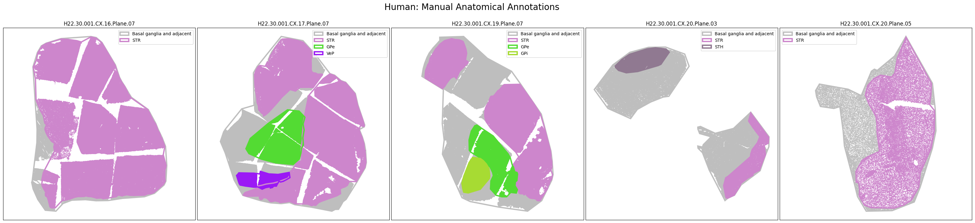
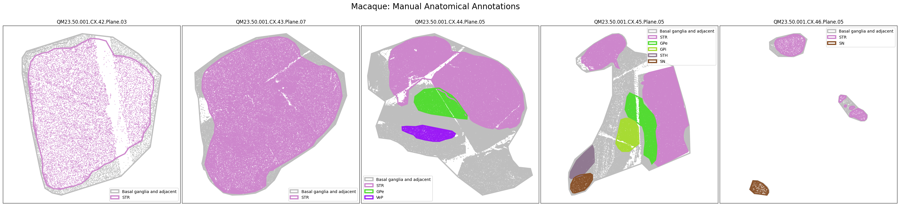
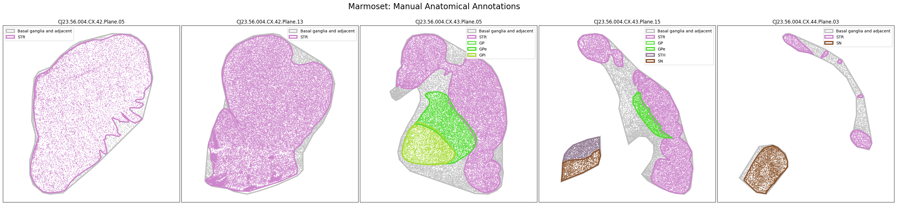
The dataset includes polygons outlining select regions of the Basal Ganglia, which can be plotted over slab coordinates. These polygon annotations were manually drawn using a combination of taxonomy cell types, select gene expression from the spatial transcriptomics gene panel, and cell segmentation stains with best attempts made to be consistent across species and planes. Manual annotations include the striatum (STR; encompasses the caudate, putamen, nucleus accumbens, and olfactory tubercle), the globus pallidus (GP) and it’s nested subregions the external (GPe) and internal (GPi) segments, the ventral pallidum (VeP), the substantia nigra (SN), and the subthalamic nucleus (STH). However, please note that these polygons are not derived from registration to the Harmonized Ontology of Mammalian Brain Anatomy (HOMBA). They should instead be used as cellular groupings to orient the user in the anatomical context of the spatial transcriptomics data and subset the data into more manageable, anatomically-related chunks. These polygons are provided in geojson format, and here we use the associated geojson python package to load the jsons for use in our visualization.

First though, we load the term set for these data. While these geojsons are manually drawn and not derived from the HOMBA, we do use the abbreviations and colors associated with these structures through their DHBA identifier when such an identifier exists. These colorings match those of the previous HMBA-BG 10X tutorial. We load these colors and identifiers below.

value_sets = abc_cache.get_metadata_dataframe(
    directory='HMBA-MERSCOPE-QM23.50.001-BG',
    file_name='value_sets',
).set_index('label')
pred = value_sets['field'] == 'parcellation_term_symbol'
parcellation_terms = value_sets[pred].copy()
parcellation_terms

value_sets.csv: 100%|██████████| 3.79k/3.79k [00:00<00:00, 64.0kMB/s]

	table	field	description	order	external_identifier	parent_label	color_hex_triplet
label
Basal ganglia and adjacent	path	parcellation_term_symbol	Basal ganglia and adjacent	1	basal_ganglia_and_adjacent	NaN	#BEBEBE
STR	path	parcellation_term_symbol	striatum	2	DHBA:10333	Basal ganglia and adjacent	#cd86cc
GP	path	parcellation_term_symbol	globus pallidus	3	DHBA:10342	Basal ganglia and adjacent	#7AE361
GPe	path	parcellation_term_symbol	external segment of globus pallidus	4	DHBA:10343	Basal ganglia and adjacent	#53DB33
GPi	path	parcellation_term_symbol	internal segment of globus pallidus	5	DHBA:10344	Basal ganglia and adjacent	#A7DB33
VeP	path	parcellation_term_symbol	ventral pallidus	6	DHBA:10345	Basal ganglia and adjacent	#9b19f5
STH	path	parcellation_term_symbol	subthalamic nucleus	7	DHBA:10466	Basal ganglia and adjacent	#907991
SN	path	parcellation_term_symbol	substantia nigra	8	DHBA:12251	Basal ganglia and adjacent	#89522A

We define two functions that will be used in our plotting of the geojsons. The first overplots the geojson over the specified plot, handling the different kinds of geojson shapes/polygons. The second loads the data based on the appropriate slab and species provided.

def plot_geo_data(geo_data: dict, ax: plt.Axes, terms=parcellation_terms):
    """Plot a geojson polygon over the input axis.

    Parameters
    ----------
    geo_data: dict
        Geojson formatted dictionary containing Polygons to plot.
    ax: matplotlib.pyplot.axis
        Axis object to plot the geojson data over.
    terms: pandas.DataFrame
        Term list containing the colors and orders for the parcellation, brain region terms. 
    """
    if geo_data is None:
        return None
    # If the geo_data is a FeatureCollection, we need to iterate over its
    # features and plot each one.
    if geo_data['type'] == 'FeatureCollection':
        for sub_data in geo_data['features']:
            plot_geo_data(sub_data, ax)
    elif geo_data['type'] == 'Feature':
        geometry_data = geo_data['geometry']
        name = geo_data['properties']['label']
        color = terms.loc[name, 'color_hex_triplet'] # Get the color for this object from the term list.
        # If the geometry is a GeometryCollection, we need to iterate over its
        # geometries that make up the complete feature.
        if geometry_data['type'] == 'GeometryCollection':
            for idx, geometry in enumerate(geometry_data['geometries']):
                coords = np.array(list(geojson.coords(geometry)))
                # Only label the first geometry in the collection. Others
                # will be plotted without a label to avoid duplicate legend entries.
                if idx == 0:
                    ax.fill(coords[:, 0],
                            coords[:, 1],
                            edgecolor=color,
                            fill=False,
                            linewidth=3,
                            label=name)
                else:
                    ax.fill(coords[:, 0],
                            coords[:, 1],
                            edgecolor=color,
                            fill=False,
                            linewidth=3)
        else:
            coords = np.array(list(geojson.coords(geometry_data)))
            try:
                ax.fill(coords[:, 0],
                        coords[:, 1],
                        edgecolor=color,
                        fill=False,
                        linewidth=3,
                        label=name)
            except ValueError as e:
                import pdb; pdb.set_trace()
    else:
        print("unknown data", geo_data)

def get_polygons(slab_name: str, species: str) -> dict:
    """Load the geojson polygons for the specified slab and species.

    Parameters
    ----------
    slab_name: str
        Name of the slab to load.
    species: str
        Species of the slab, one of 'macaque', 'marmoset', or 'human'.

    Returns
    -------
    dict
        Geojson formatted dictionary containing the polygons for the specified slab and species.
    """

    if species == 'macaque':
        base_dir = 'HMBA-MERSCOPE-QM23.50.001-BG'
    elif species == 'marmoset':
        base_dir = 'HMBA-Xenium-CJ23.56.004-BG'
    elif species == 'human':
        base_dir = 'HMBA-MERSCOPE-H22.30.001-BG'
    else:
        raise ValueError('Invalid species')

    file_path = abc_cache.get_file_path(directory=base_dir, file_name=slab_name)
    if not file_path.exists():
        return None

    with open(file_path) as jfile:
        data = json.load(jfile)
    
    return data

Manual anatomical annotations

Using the manually drawn anatomical polygons described above, each cell was assigned membership in the annotated anatomical regions. The tables we load below contain boolean columns denoting which anatomical regions the cell could be considered a member of. Note that a given cell can belong to multiple different anatomical annotations as the polygons overlap and can be subsets of each other. For instance, all cells in this release are within the “Basal Ganglia and adjacent” annotation, and most cells in either “GPe” or “GPi” are within the parent annotation “GP”. The final column, parcellation_term_symbol is a single value representing a single unique assignment to a structure based on selecting from STH in reverse order of the columns, keeping the first True assignment. For this notebook, we will use only the parcellation_term_symbol to plot our data.

human_cell_anatomical_annotations = abc_cache.get_metadata_dataframe(
    directory='HMBA-MERSCOPE-H22.30.001-BG',
    file_name='cell_anatomical_annotations'
).set_index('cell_label')
human_cell_anatomical_annotations.head()

cell_anatomical_annotations.csv: 100%|██████████| 448M/448M [00:16<00:00, 27.9MMB/s]    

	Basal ganglia and adjacent	STR	GP	GPe	GPi	VeP	SN	STH	parcellation_term_symbol
cell_label
1321115602_1-20250227	True	True	False	False	False	False	False	False	STR
1321115602_2-20250227	True	True	False	False	False	False	False	False	STR
1321115602_3-20250227	True	True	False	False	False	False	False	False	STR
1321115602_4-20250227	True	True	False	False	False	False	False	False	STR
1321115602_5-20250227	True	True	False	False	False	False	False	False	STR

macaque_cell_anatomical_annotations = abc_cache.get_metadata_dataframe(
    directory='HMBA-MERSCOPE-QM23.50.001-BG',
    file_name='cell_anatomical_annotations'
).set_index('cell_label')
macaque_cell_anatomical_annotations.head()

cell_anatomical_annotations.csv: 100%|██████████| 275M/275M [00:10<00:00, 26.3MMB/s]    

	Basal ganglia and adjacent	STR	GP	GPe	GPi	VeP	SN	STH	parcellation_term_symbol
cell_label
1291813781_1-20250227	True	False	False	False	False	False	False	False	Basal ganglia and adjacent
1291813781_2-20250227	True	False	False	False	False	False	False	False	Basal ganglia and adjacent
1291813781_3-20250227	True	False	False	False	False	False	False	False	Basal ganglia and adjacent
1291813781_4-20250227	True	False	False	False	False	False	False	False	Basal ganglia and adjacent
1291813781_5-20250227	True	False	False	False	False	False	False	False	Basal ganglia and adjacent

marmoset_cell_anatomical_annotations = abc_cache.get_metadata_dataframe(
    directory='HMBA-Xenium-CJ23.56.004-BG',
    file_name='cell_anatomical_annotations'
).set_index('cell_label')
marmoset_cell_anatomical_annotations.head()

cell_anatomical_annotations.csv:   0%|          | 0.00/116M [00:00<?, ?MB/s]

cell_anatomical_annotations.csv: 100%|██████████| 116M/116M [00:04<00:00, 23.3MMB/s]   

	Basal ganglia and adjacent	STR	GP	GPe	GPi	VeP	SN	STH	parcellation_term_symbol
cell_label
1382042951_abmkfncc-1-20250227	True	False	False	False	False	False	False	False	Basal ganglia and adjacent
1382042951_abmmdgea-1-20250227	True	False	False	False	False	False	False	False	Basal ganglia and adjacent
1382042951_abmojfce-1-20250227	True	False	False	False	False	False	False	False	Basal ganglia and adjacent
1382042951_abmomnim-1-20250227	True	False	False	False	False	False	False	False	Basal ganglia and adjacent
1382042951_aeiamgga-1-20250227	True	True	False	False	False	False	False	False	STR

Below, we define a function to extract color and order information from the value_set table for each anatomical parcellation term. This will allow us to plot the color of the anatomical region we assigned each cell to using the manually drawn, geojson polygons.

def extract_value_set(cell_metadata_df: pd.DataFrame, input_value_set: pd.DataFrame, input_value_set_label: str):
    """Add color and order columns to the cell metadata dataframe based on the input
    value set.

    Columns are added as {input_value_set_label}_color and {input_value_set_label}_order.

    Parameters
    ----------
    cell_metadata_df : pd.DataFrame
        DataFrame containing cell metadata.
    input_value_set : pd.DataFrame
        DataFrame containing the value set information.
    input_value_set_label : str
        The the column name to extract color and order information for. will be added to the cell metadata.
    """
    cell_metadata_df[f'{input_value_set_label}_color'] = input_value_set[
        input_value_set['field'] == input_value_set_label
    ].loc[cell_metadata_df[input_value_set_label]]['color_hex_triplet'].values
    cell_metadata_df[f'{input_value_set_label}_order'] = input_value_set[
        input_value_set['field'] == input_value_set_label
    ].loc[cell_metadata_df[input_value_set_label]]['order'].values

Merge the manual annotation information into the cell meatadata tables and add in the color and ordering information.

human_cell_metadata = human_cell_metadata.join(
    human_cell_anatomical_annotations[['parcellation_term_symbol']]
)
macaque_cell_metadata = macaque_cell_metadata.join(
    macaque_cell_anatomical_annotations[['parcellation_term_symbol']]
)
marmoset_cell_metadata = marmoset_cell_metadata.join(
    marmoset_cell_anatomical_annotations[['parcellation_term_symbol']]
)
extract_value_set(human_cell_metadata, parcellation_terms, 'parcellation_term_symbol')
extract_value_set(macaque_cell_metadata, parcellation_terms, 'parcellation_term_symbol')
extract_value_set(marmoset_cell_metadata, parcellation_terms, 'parcellation_term_symbol')

human_cell_metadata = human_cell_metadata.sort_values(by='parcellation_term_symbol_order')
macaque_cell_metadata = macaque_cell_metadata.sort_values(by='parcellation_term_symbol_order')
marmoset_cell_metadata = marmoset_cell_metadata.sort_values(by='parcellation_term_symbol_order')

# clean up memory
del human_cell_anatomical_annotations
del macaque_cell_anatomical_annotations
del marmoset_cell_anatomical_annotations

Plotting the Slabs

We define a helper function plot_slabs to visualize the cells for a specified set of slabs either by colorized metadata or gene expression. The code also allows for plotting the annotation polygons over the data if requested. This function can be used to plot individual frames as well.

def plot_slabs(
    df: pd.DataFrame,
    feature: str,
    slab_list: List[str],
    species: str,
    cmap: Optional[plt.Colormap] = None,
    fig_width: float = 40,
    fig_height: float = 8,
    plot_polygons: bool = False,
    point_size: float = 1.0,
    fix_bounds: bool = False
) -> Tuple[plt.Figure, np.ndarray]:
    """Plot spatial transcriptomics data.

    Parameters
    ----------
    df: pandas.DataFrame
        cell metadata data frame with x,y locations to plot.
    feature: str
        Expression value or color column to plot.
    slab_list: List[str]
        List of slab_plane ids to plot.
    species: str
        Species to plot (human, macaque, marmoset).
    cmap: matplotlib.colors.Colormap
        Colormap for expression features.
    fig_width: int
        Width of the plotted figure.
    fig_height: int
        Height of the plotted figure.
    plot_polygons: bool
        Overplot geojson polygons. Note that these are note available for human
        and this should be set to False.
    point_size: float
        Size of the points to plot.
    fix_bounds: bool
        If True, fix the x and y bounds across all slabs to be the same.
    """
    if isinstance(slab_list, str):
        slab_list = [slab_list]

    fig, ax = plt.subplots(1, len(slab_list))
    fig.set_size_inches(fig_width, fig_height)

    if len(slab_list) == 1:
        ax = [ax]

    if 'x' in df.columns:
        x_col = 'x'
    elif 'x_slab_mm' in df.columns:
        x_col = 'x_slab_mm'
    if 'y' in df.columns:
        y_col = 'y'
    elif 'y_slab_mm' in df.columns:
        y_col = 'y_slab_mm'

    if fix_bounds:
        x_min = df[x_col].min() * 0.8
        x_max = df[x_col].max() * 1.2
        y_min = df[y_col].min() * 0.8
        y_max = df[y_col].max() * 1.2

    for idx, slab in enumerate(slab_list):

        if 'slab_plane_label' in df.columns:
            filtered = df[df['slab_plane_label'] == slab]
        elif 'brain_section_label' in df.columns:
            filtered = df[df['brain_section_label'] == slab]
        
        xx = filtered[x_col]
        yy = filtered[y_col]
        vv = filtered[feature]
        
        if cmap is not None:
            ax[idx].scatter(xx, yy, s=point_size, c=vv, marker='.', cmap=cmap)
        else:
            
            ax[idx].scatter(xx, yy, s=point_size, c=vv, marker=".")

        if plot_polygons:
            plot_geo_data(get_polygons(slab, species=species), ax[idx])
            
        ax[idx].axis('equal')
        if fix_bounds:
            ax[idx].set_ylim(y_min, y_max)
            ax[idx].set_xlim(x_min, x_max)
        ylim = ax[idx].get_ylim()
        ax[idx].set_ylim(ylim[1], ylim[0])
        ax[idx].set_xticks([])
        ax[idx].set_yticks([])
        
        ax[idx].set_title(slab)
        ax[idx].legend(loc=0)
        
    plt.subplots_adjust(wspace=0.01, hspace=0.01)
    return fig, ax

Displaying the manual anatomical annotations.

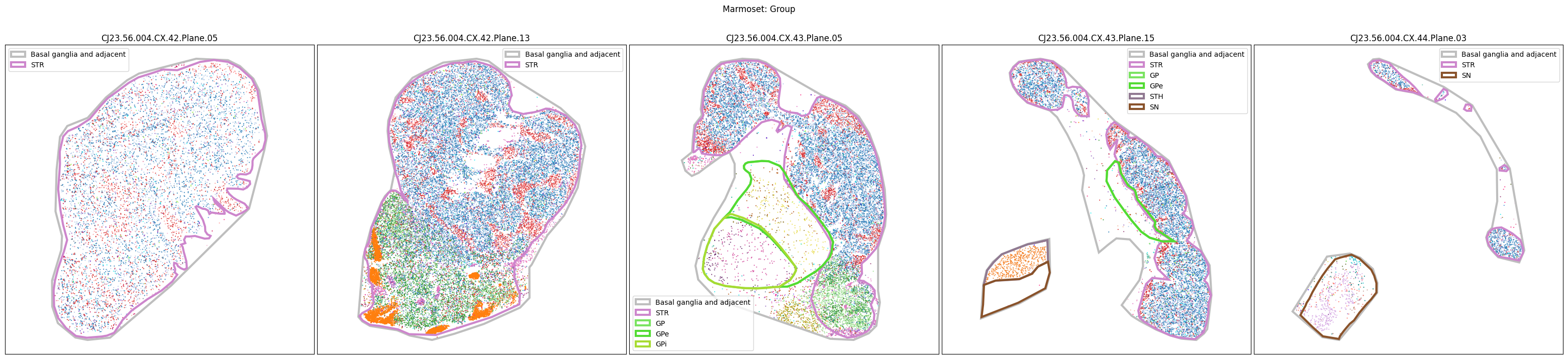
We now have a set of cells in x,y slab coordinates and metadata on the anatomical regions these cells have been manually annotated as members of. Below we plot the cells using the colors as defined in our term set, displaying the cells by manually annotated regions of the Basal Ganglia.

human_slab_list = [
    'H22.30.001.CX.16.Plane.07', 'H22.30.001.CX.17.Plane.07',
    'H22.30.001.CX.19.Plane.07', 'H22.30.001.CX.20.Plane.03', 'H22.30.001.CX.20.Plane.05'
]
color_type = 'parcellation_term_symbol_color'
fig, ax = plot_slabs(
    human_cell_metadata,
    color_type,
    human_slab_list,
    species='human',
    plot_polygons=True,
)
fig.suptitle(f'Human: Manual Anatomical Annotations', size=20)
plt.show()

H22.30.001.CX.16.Plane.07.geojson: 100%|██████████| 5.47k/5.47k [00:00<00:00, 70.9kMB/s]
H22.30.001.CX.17.Plane.07.geojson: 100%|██████████| 8.08k/8.08k [00:00<00:00, 158kMB/s]
H22.30.001.CX.19.Plane.07.geojson: 100%|██████████| 5.97k/5.97k [00:00<00:00, 63.6kMB/s]
H22.30.001.CX.20.Plane.03.geojson: 100%|██████████| 3.00k/3.00k [00:00<00:00, 51.0kMB/s]
H22.30.001.CX.20.Plane.05.geojson: 100%|██████████| 2.35k/2.35k [00:00<00:00, 49.2kMB/s]

macaque_slab_list = [
    'QM23.50.001.CX.42.Plane.03', 'QM23.50.001.CX.43.Plane.07', 'QM23.50.001.CX.44.Plane.05',
    'QM23.50.001.CX.45.Plane.05', 'QM23.50.001.CX.46.Plane.05'
]
color_type = 'parcellation_term_symbol_color'
fig, ax = plot_slabs(
    macaque_cell_metadata,
    color_type,
    macaque_slab_list,
    species='macaque',
    plot_polygons=True
)
fig.suptitle(f'Macaque: Manual Anatomical Annotations', size=20)
plt.show()

QM23.50.001.CX.42.Plane.03.geojson: 100%|██████████| 2.33k/2.33k [00:00<00:00, 20.3kMB/s]
QM23.50.001.CX.43.Plane.07.geojson: 100%|██████████| 2.99k/2.99k [00:00<00:00, 59.2kMB/s]
QM23.50.001.CX.44.Plane.05.geojson: 100%|██████████| 5.53k/5.53k [00:00<00:00, 85.2kMB/s]
QM23.50.001.CX.45.Plane.05.geojson: 100%|██████████| 6.83k/6.83k [00:00<00:00, 139kMB/s]
QM23.50.001.CX.46.Plane.05.geojson: 100%|██████████| 5.00k/5.00k [00:00<00:00, 59.1kMB/s]

marmoset_slab_list = [
    'CJ23.56.004.CX.42.Plane.05', 'CJ23.56.004.CX.42.Plane.13', 'CJ23.56.004.CX.43.Plane.05',
    'CJ23.56.004.CX.43.Plane.15', 'CJ23.56.004.CX.44.Plane.03'
]
color_type = 'parcellation_term_symbol_color'
fig, ax = plot_slabs(
    marmoset_cell_metadata,
    color_type,
    marmoset_slab_list,
    species='marmoset',
    plot_polygons=True
)
fig.suptitle(f'Marmoset: Manual Anatomical Annotations', size=20)
plt.show()

CJ23.56.004.CX.42.Plane.05.geojson: 100%|██████████| 6.43k/6.43k [00:00<00:00, 89.7kMB/s]
CJ23.56.004.CX.42.Plane.13.geojson: 100%|██████████| 6.54k/6.54k [00:00<00:00, 124kMB/s]
CJ23.56.004.CX.43.Plane.05.geojson: 100%|██████████| 12.2k/12.2k [00:00<00:00, 178kMB/s]
CJ23.56.004.CX.43.Plane.15.geojson: 100%|██████████| 9.98k/9.98k [00:00<00:00, 167kMB/s]
CJ23.56.004.CX.44.Plane.03.geojson: 100%|██████████| 5.77k/5.77k [00:00<00:00, 104kMB/s]

Taxonomy mapping

Now that we have our base functions for plotting set up and we’ve exercised them using the parcellation colors, let’s load the taxonomy information so that we can plot the spatial locations of various cell types. Below, we load and merge all the information we need to plot cell colors and taxonomy as done in the previous HMBA-BG tutorials.

cluster = abc_cache.get_metadata_dataframe(
    directory='HMBA-BG-taxonomy-CCN20250428',
    file_name='cluster',
    dtype={'number_of_cells': 'Int64'}
).rename(columns={'label': 'cluster_annotation_term_label'}).set_index('cluster_annotation_term_label')
cluster_annotation_term_set = abc_cache.get_metadata_dataframe(
    directory='HMBA-BG-taxonomy-CCN20250428',
    file_name='cluster_annotation_term_set'
).rename(columns={'label': 'cluster_annotation_term_label'})

cluster_annotation_term = abc_cache.get_metadata_dataframe(
    directory='HMBA-BG-taxonomy-CCN20250428',
    file_name='cluster_annotation_term',
).rename(columns={'label': 'cluster_annotation_term_label'}).set_index('cluster_annotation_term_label')

cluster_to_cluster_annotation_membership = abc_cache.get_metadata_dataframe(
    directory='HMBA-BG-taxonomy-CCN20250428',
    file_name='cluster_to_cluster_annotation_membership',
).set_index('cluster_annotation_term_label')
membership_with_cluster_info = cluster_to_cluster_annotation_membership.join(
    cluster.reset_index().set_index('cluster_alias')[['number_of_cells']],
    on='cluster_alias'
)
membership_with_cluster_info = membership_with_cluster_info.join(cluster_annotation_term, rsuffix='_anno_term').reset_index()
membership_groupby = membership_with_cluster_info.groupby(
    ['cluster_alias', 'cluster_annotation_term_set_name']
)

cluster_annotation_term_set = abc_cache.get_metadata_dataframe(
    directory='HMBA-BG-taxonomy-CCN20250428',
    file_name='cluster_annotation_term_set'
).rename(columns={'label': 'cluster_annotation_term_label'})

# term_sets = abc_cache.get_metadata_dataframe(directory='WHB-taxonomy', file_name='cluster_annotation_term_set').set_index('label')
cluster_details = membership_groupby['cluster_annotation_term_name'].first().unstack()
cluster_order = membership_groupby['term_order'].first().unstack()
cluster_order.sort_values(['Neighborhood', 'Class', 'Subclass', 'Group', 'Cluster'], inplace=True)
cluster_order.rename(
    columns={'Neighborhood': 'Neighborhood_order',
             'Class': 'Class_order',
             'Subclass': 'Subclass_order',
             'Group': 'Group_order',
             'Cluster': 'Cluster_order'},
    inplace=True
)

cluster_colors = membership_groupby['color_hex_triplet'].first().unstack()
cluster_colors = cluster_colors[cluster_annotation_term_set['name']]
cluster_colors.sort_values(
    ['Neighborhood', 'Class', 'Subclass', 'Group', 'Cluster'],
    inplace=True
)

Each of the three species has been mapped to the HMBA 10X taxonomy using MapMyCells. Below, we load the mapping of each cell to a taxonomy cluster. This mapping is the entry point into the taxonomy.

Again, we load each species.

human_cell_to_cluster = abc_cache.get_metadata_dataframe(
    directory='HMBA-MERSCOPE-H22.30.001-BG',
    file_name='cell_to_cluster_membership'
).set_index('cell_label')

macaque_cell_to_cluster = abc_cache.get_metadata_dataframe(
    directory='HMBA-MERSCOPE-QM23.50.001-BG',
    file_name='cell_to_cluster_membership',
).set_index('cell_label')

marmoset_cell_to_cluster = abc_cache.get_metadata_dataframe(
    directory='HMBA-Xenium-CJ23.56.004-BG',
    file_name='cell_to_cluster_membership',
).set_index('cell_label')

cell_to_cluster_membership.csv: 100%|██████████| 310M/310M [00:14<00:00, 22.0MMB/s]    
cell_to_cluster_membership.csv: 100%|██████████| 195M/195M [00:07<00:00, 26.6MMB/s]    
cell_to_cluster_membership.csv: 100%|██████████| 88.1M/88.1M [00:03<00:00, 25.7MMB/s]  

The spatial data are registered to an extended version of the taxonomy that contains clusters that are considered Adjacent to the Basal Ganglia. These are cell types that are present in the data but are not considered part of the basal ganglia. These clusters are mapped into a Group, Subclass, Class, and Neighborhood in a single path of the taxonomy called Adjacent. The release consensus taxonomy does not explicitly contain this taxon. Any cell in a cluster that would be annotated into Adjacent, will end up being NaN in the joins between the clusters and the taxonomy. We thus fill in these NaNs, assigning any cell that was not mapped into to a group in the taxonomy an Adjacent cell type at all levels with a grey color. We give these Adjacent taxons an ordering at the very end of the set of taxons at each level.”

Although the BG Consensus Taxonomy is intended to be specific to BG cell types, when the data were sampled for the snRNA-Seq reference, some cells from adjacent non-BG regions were included. Because these cells originated from non-BG regions, we did not assign them a cell type identity (i.e. a label at the Group, Subclass, etc. levels). However, because 1) our spatial transcriptomics datasets also contain cells from adjacent non-BG regions, and 2) MapMyCells requires every cell to be assigned a label from the reference, including Adjacent cells in the reference decreases spurious mapping results in BG-adjacent regions. Adjacent cells are included in the release data for completeness, where they are labeled as “Adjacent” at all taxonomy levels. When visualizing cells in BG regions, we recommend filtering them out.

def fill_adjacent_data(input_df: pd.DataFrame) -> pd.DataFrame:
    output_df = input_df.fillna(
        {'cluster_alias': 'Adjacent',
         'cluster_label': 'Adjacent',
         'Class': 'Adjacent',
         'Cluster': 'Adjacent',
         'Group': 'Adjacent',
         'Neighborhood': 'Adjacent',
         'Subclass': 'Adjacent',
         'Neighborhood_color': '#808080',
         'Class_color': '#808080',
         'Subclass_color': '#808080',
         'Group_color': '#808080',
         'Cluster_color': '#808080',
         'Neighborhood_order': cluster_order.max()['Neighborhood_order'] + 1,
         'Class_order': cluster_order.max()['Class_order'] + 1,
         'Subclass_order': cluster_order.max()['Subclass_order'] + 1,
         'Group_order': cluster_order.max()['Group_order'] + 1,
         'Cluster_order': cluster_order.max()['Cluster_order'] + 1,
        }
    )
    return output_df.astype(
        {
            'Neighborhood_order': 'int',
            'Class_order': 'int',
            'Subclass_order': 'int',
            'Group_order': 'int',
            'Cluster_order': 'int',
        }
    )

Now we merge the cell type classification colors and order into our metadata for each species.

human_cell_metadata = human_cell_metadata.join(human_cell_to_cluster)
human_cell_metadata = human_cell_metadata.join(cluster_details, on='cluster_alias')
human_cell_metadata = human_cell_metadata.join(cluster_colors, on='cluster_alias', rsuffix='_color')
human_cell_metadata = human_cell_metadata.join(cluster_order, on='cluster_alias')
human_cell_metadata = fill_adjacent_data(human_cell_metadata)

del human_cell_to_cluster

human_cell_metadata.head()

	brain_section_label	brain_section_barcode	segmentation_job_id	x_experiment	y_experiment	qc_pass	dataset_label	feature_matrix_label	abc_sample_id	brain_section_barcode_specimen	...	Neighborhood_color	Class_color	Subclass_color	Group_color	Cluster_color	Class_order	Cluster_order	Group_order	Neighborhood_order	Subclass_order
cell_label
1384732733_104390-20250227	H22.30.001.CX.20.02.03.01	1384732733	sis_cellpose_v1	9122.90000	2747.79320	True	HMBA-MERSCOPE-H22.30.001-BG	MERSCOPE-H22.30.001-BG	1bb3cc09-224a-412b-8a09-59438370c64f	1384732733	...	#a8afa5	#a8afa5	#B97300	#B97300	#8b3406	4	261	15	1	11
1326494670_42591-20250227	H22.30.001.CX.17.07.07.02	1326494670	sis_cellpose_v1	623.67487	903.07245	True	HMBA-MERSCOPE-H22.30.001-BG	MERSCOPE-H22.30.001-BG	3d211210-71d6-47f9-a88f-946f56c9ba8c	1326494670	...	#a8afa5	#594a26	#594a26	#66391F	#a9de1a	3	142	9	1	7
1326494670_42590-20250227	H22.30.001.CX.17.07.07.02	1326494670	sis_cellpose_v1	498.75037	902.13605	True	HMBA-MERSCOPE-H22.30.001-BG	MERSCOPE-H22.30.001-BG	e059d8e7-29ce-48f9-9105-df1c9ba966c1	1326494670	...	#a8afa5	#594a26	#594a26	#66391F	#7db606	3	144	9	1	7
1326494670_42589-20250227	H22.30.001.CX.17.07.07.02	1326494670	sis_cellpose_v1	421.28458	900.51600	True	HMBA-MERSCOPE-H22.30.001-BG	MERSCOPE-H22.30.001-BG	c017a97b-0c6a-41b0-b4b5-6f99e4a5759d	1326494670	...	#a8afa5	#594a26	#f5e689	#f5e689	#8c2187	3	210	12	1	8
1326494670_42588-20250227	H22.30.001.CX.17.07.07.02	1326494670	sis_cellpose_v1	406.79843	899.12110	True	HMBA-MERSCOPE-H22.30.001-BG	MERSCOPE-H22.30.001-BG	59579c65-2336-44e4-ae2e-284dd9766ed4	1326494670	...	#a8afa5	#594a26	#594a26	#594a26	#6af4cf	3	161	10	1	7

5 rows × 51 columns

Load the Macaque and Marmoset data in the same way.

macaque_cell_to_cluster = abc_cache.get_metadata_dataframe(
    directory='HMBA-MERSCOPE-QM23.50.001-BG',
    file_name='cell_to_cluster_membership',
).set_index('cell_label')

macaque_cell_metadata = macaque_cell_metadata.join(macaque_cell_to_cluster)
macaque_cell_metadata = macaque_cell_metadata.join(cluster_details, on='cluster_alias')
macaque_cell_metadata = macaque_cell_metadata.join(cluster_colors, on='cluster_alias', rsuffix='_color')
macaque_cell_metadata = macaque_cell_metadata.join(cluster_order, on='cluster_alias')
macaque_cell_metadata = fill_adjacent_data(macaque_cell_metadata)

del macaque_cell_to_cluster

macaque_cell_metadata.head()

	brain_section_label	brain_section_barcode	segmentation_job_id	x_experiment	y_experiment	qc_pass	dataset_label	feature_matrix_label	abc_sample_id	brain_section_barcode_specimen	...	Neighborhood_color	Class_color	Subclass_color	Group_color	Cluster_color	Class_order	Cluster_order	Group_order	Neighborhood_order	Subclass_order
cell_label
1291813781_1-20250227	QM23.50.001.CX.44.03.07.02	1291813781	sis_cellpose_v1	6328.8564	271.7173	False	HMBA-MERSCOPE-QM23.50.001-BG	MERSCOPE-QM23.50.001-BG	NaN	1291813781	...	#19613b	#d0b83c	#253c8c	#ff9896	#681364	10	1289	55	3	32
1291812338_13027-20250227	QM23.50.001.CX.43.01.11.03	1291812338	sis_cellpose_v1	8314.5330	2671.2260	True	HMBA-MERSCOPE-QM23.50.001-BG	MERSCOPE-QM23.50.001-BG	6de019e9-4c63-470b-b474-3b8d23947d84	1291812338	...	#19613b	#d0b83c	#79bdf4	#e377c2	#8f8307	10	1335	57	3	33
1291812338_13026-20250227	QM23.50.001.CX.43.01.11.03	1291812338	sis_cellpose_v1	8180.6080	2670.6003	True	HMBA-MERSCOPE-QM23.50.001-BG	MERSCOPE-QM23.50.001-BG	288bf294-b18b-42e9-b0fc-84234c008a8a	1291812338	...	#19613b	#d0b83c	#1655f2	#d62728	#307e06	10	1166	52	3	31
1291812338_13025-20250227	QM23.50.001.CX.43.01.11.03	1291812338	sis_cellpose_v1	8336.7420	2667.5422	True	HMBA-MERSCOPE-QM23.50.001-BG	MERSCOPE-QM23.50.001-BG	37da2f12-be8f-42a3-93ab-0a31ef0e4382	1291812338	...	#a8afa5	#594a26	#594a26	#66391F	#62620e	3	146	9	1	7
1291812338_13024-20250227	QM23.50.001.CX.43.01.11.03	1291812338	sis_cellpose_v1	8315.9370	2664.6123	True	HMBA-MERSCOPE-QM23.50.001-BG	MERSCOPE-QM23.50.001-BG	dca478a5-0c68-451d-a832-80e977e075cb	1291812338	...	#a8afa5	#401e66	#401e66	#195f8d	#21e5fe	1	25	1	1	1

5 rows × 51 columns

marmoset_cell_to_cluster = abc_cache.get_metadata_dataframe(
    directory='HMBA-Xenium-CJ23.56.004-BG',
    file_name='cell_to_cluster_membership',
).set_index('cell_label')

marmoset_cell_metadata = marmoset_cell_metadata.join(marmoset_cell_to_cluster)
marmoset_cell_metadata = marmoset_cell_metadata.join(cluster_details, on='cluster_alias')
marmoset_cell_metadata = marmoset_cell_metadata.join(cluster_colors, on='cluster_alias', rsuffix='_color')
marmoset_cell_metadata = marmoset_cell_metadata.join(cluster_order, on='cluster_alias')
marmoset_cell_metadata = fill_adjacent_data(marmoset_cell_metadata)

del marmoset_cell_to_cluster

marmoset_cell_metadata.head()

	brain_section_label	brain_section_barcode	segmentation_job_id	x_experiment	y_experiment	qc_pass	dataset_label	feature_matrix_label	abc_sample_id	brain_section_barcode_specimen	...	Neighborhood_color	Class_color	Subclass_color	Group_color	Cluster_color	Class_order	Cluster_order	Group_order	Neighborhood_order	Subclass_order
cell_label
1382042951_abmkfncc-1-20250227	CJ23.56.004.CX.42.01.06	1382042951	xenium_cell_segmentation_kit_v1	5923.492676	6160.654297	True	HMBA-Xenium-CJ23.56.004-BG	Xenium-CJ23.56.004-BG	c8c08d8c-5147-4d03-b6f4-ca7bf4d0b8d1	1382042951	...	#a8afa5	#594a26	#594a26	#66391F	#5a9ad6	3	158	9	1	7
1386591529_oglkpmal-1-20250227	CJ23.56.004.CX.43.01.07	1386591529	xenium_cell_segmentation_kit_v1	10066.064453	9964.978516	True	HMBA-Xenium-CJ23.56.004-BG	Xenium-CJ23.56.004-BG	899a0853-cb22-4b1f-a34c-6e2fad41acd2	1386591529	...	#a8afa5	#995C60	#995C60	#995C60	#54ca78	2	113	4	1	3
1386591529_oglkphgf-1-20250227	CJ23.56.004.CX.43.01.07	1386591529	xenium_cell_segmentation_kit_v1	10032.336914	9951.043945	True	HMBA-Xenium-CJ23.56.004-BG	Xenium-CJ23.56.004-BG	1f87149d-55fe-4081-b6da-c2bf68189e48	1386591529	...	#a8afa5	#594a26	#f5e689	#f5e689	#f222e1	3	219	12	1	8
1386591529_oglkpgff-1-20250227	CJ23.56.004.CX.43.01.07	1386591529	xenium_cell_segmentation_kit_v1	10078.684570	9936.422852	True	HMBA-Xenium-CJ23.56.004-BG	Xenium-CJ23.56.004-BG	37a9464c-9dff-4823-a36a-42bb7ca37fef	1386591529	...	#a8afa5	#a8afa5	#66493D	#66493D	#1bf6d7	4	253	14	1	10
1386591529_oglikmic-1-20250227	CJ23.56.004.CX.43.01.07	1386591529	xenium_cell_segmentation_kit_v1	9677.964844	11089.391602	True	HMBA-Xenium-CJ23.56.004-BG	Xenium-CJ23.56.004-BG	228d9fa6-bea9-4813-8c82-7285f1e5754b	1386591529	...	#a8afa5	#995C60	#CC887A	#CC887A	#80f3ea	2	130	5	1	4

5 rows × 51 columns

Merging in the taxonomy allows one to select cells by the specific taxons they are associated with, as we will see in a function we create below.

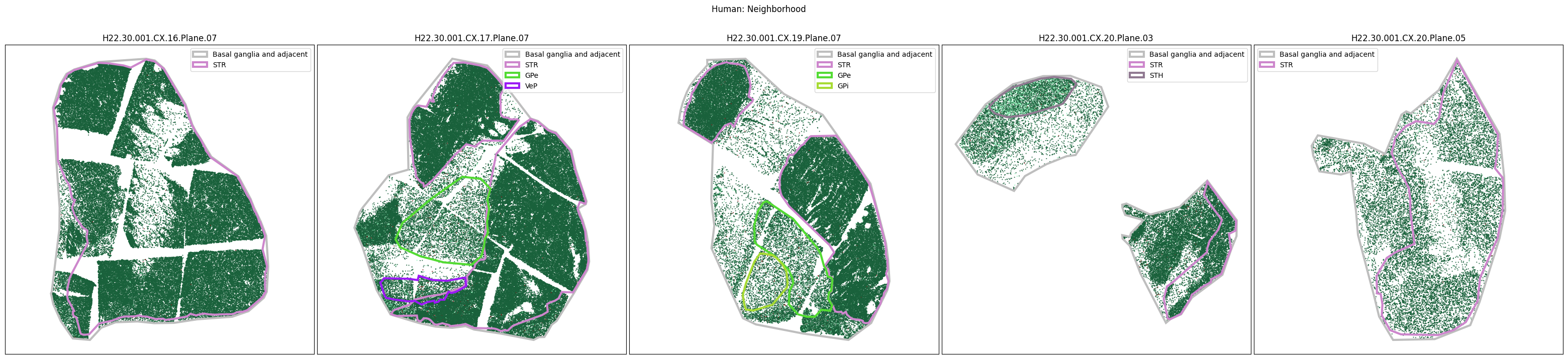
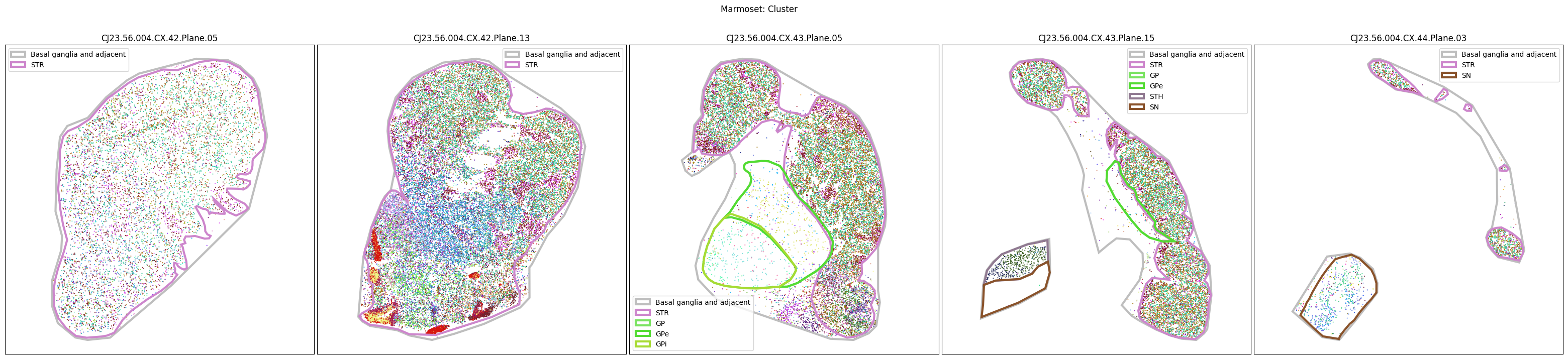
Plotting the taxonomy

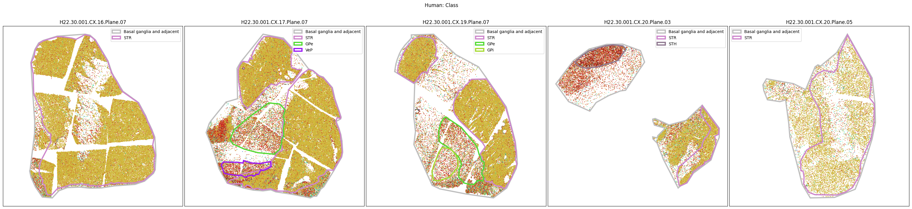
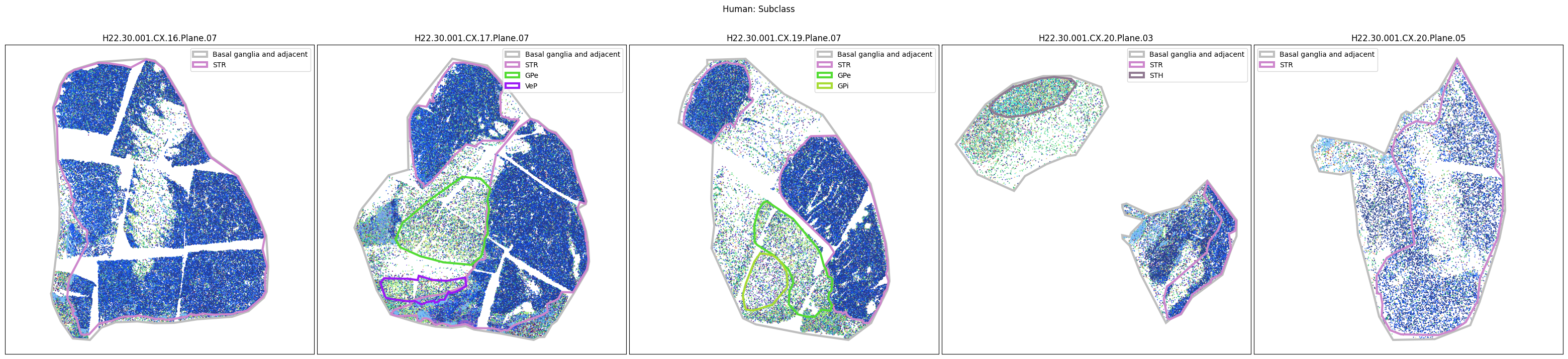
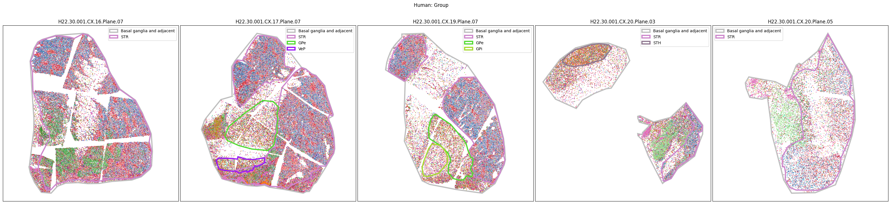
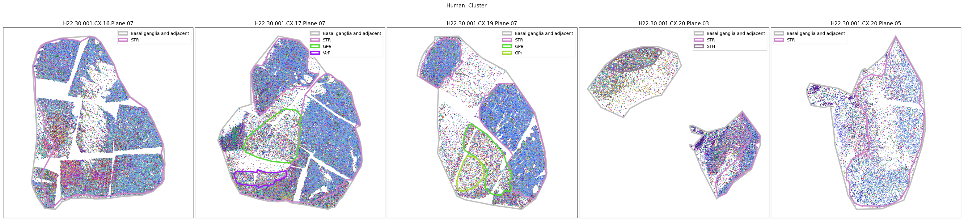
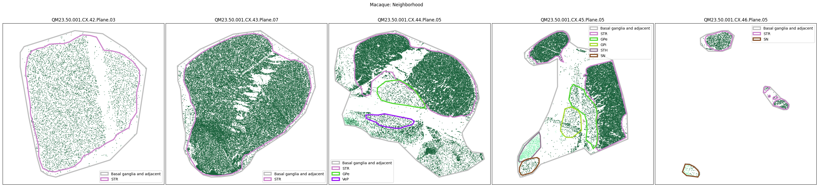
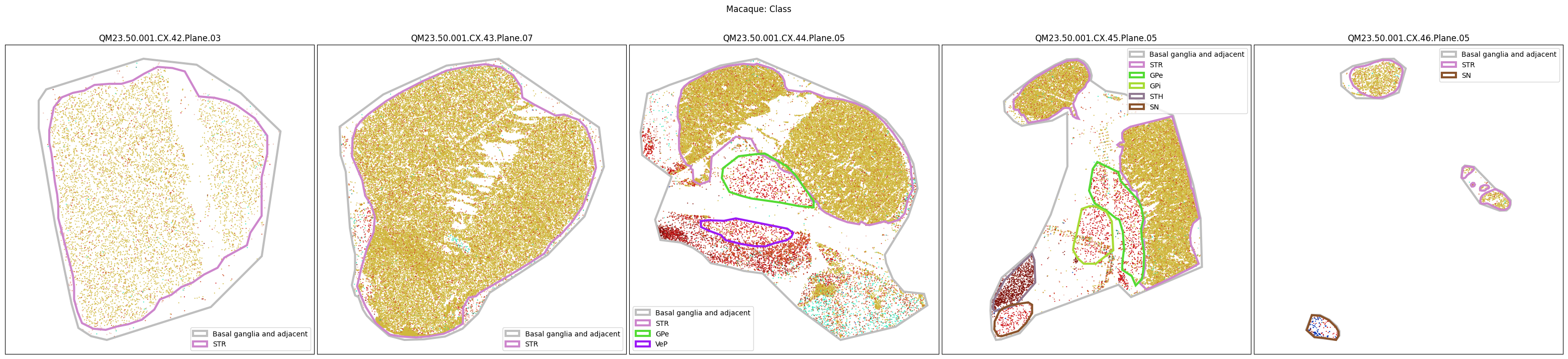
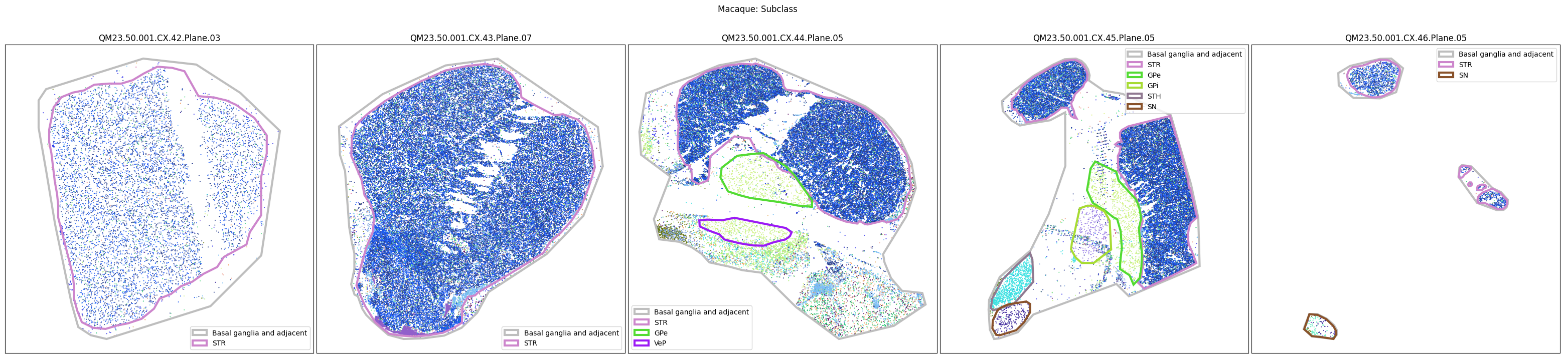
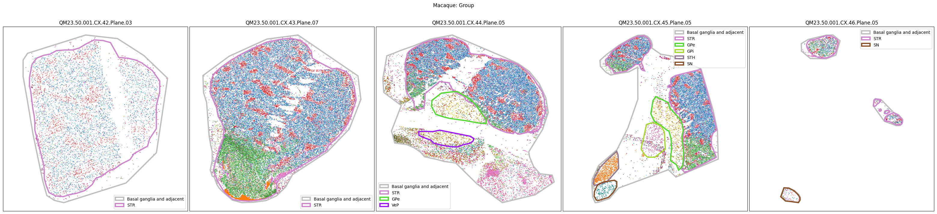
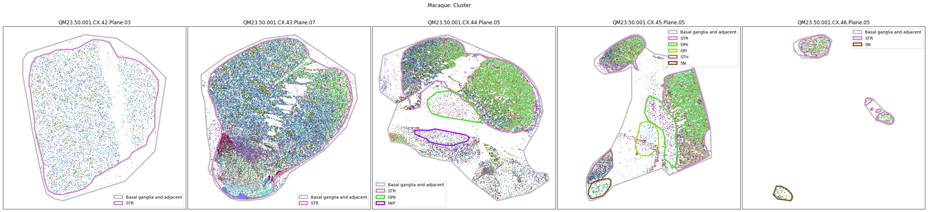
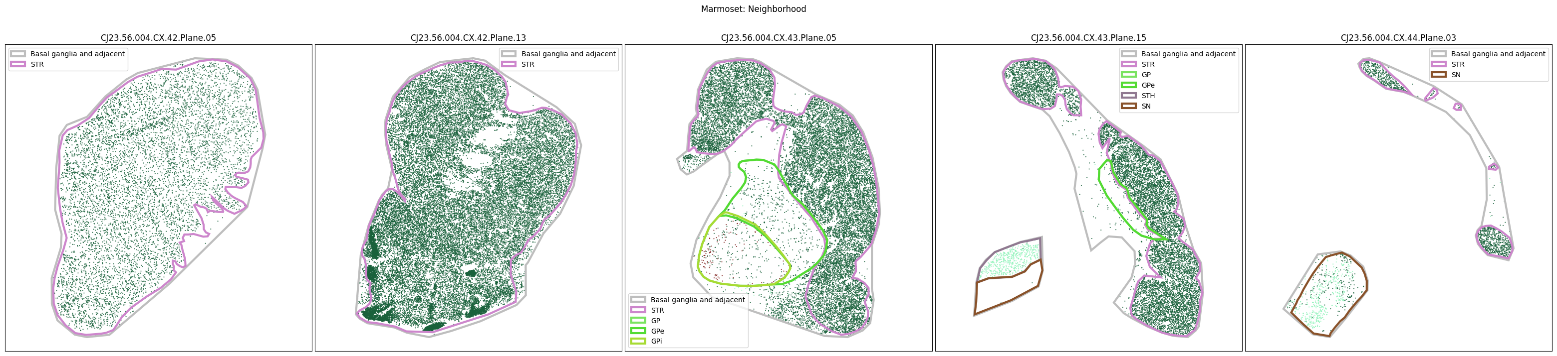
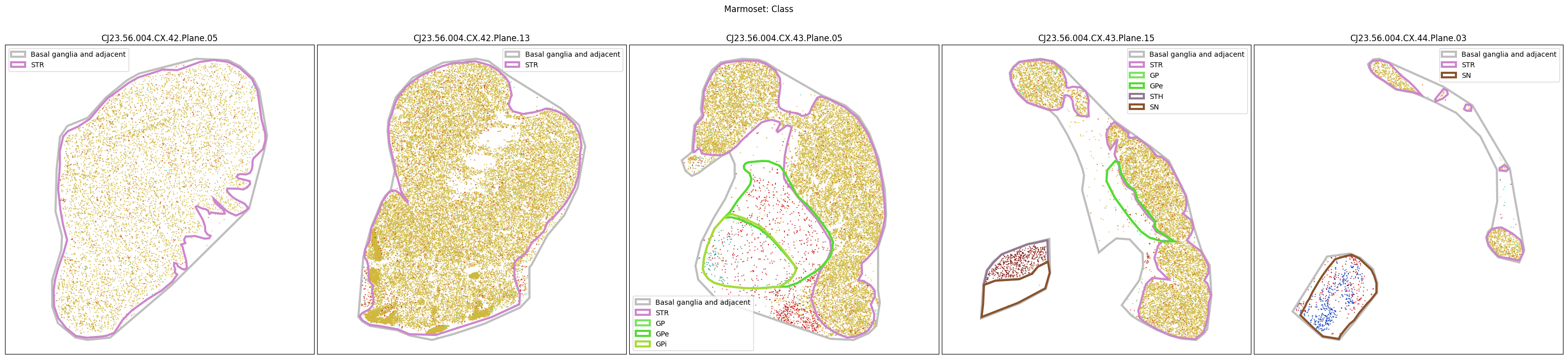
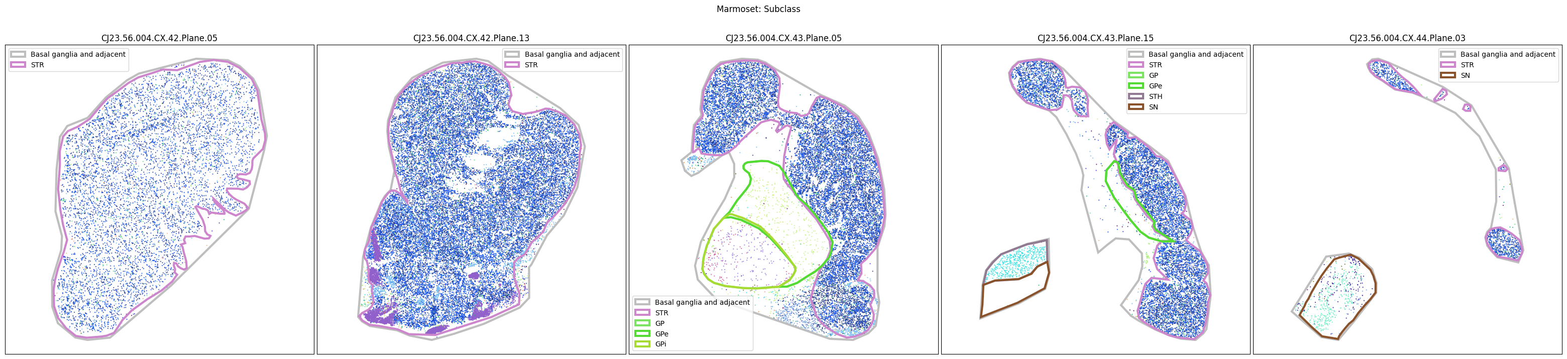
Now that the taxonomy is loaded, we plot the the cells showing the spatial locations of the cell types in the Basal Ganglia. Below we plot each species in the dataset for each of the 5 levels in the taxonomy selection using the same set of slabs we used for the above to plot the manual anatomical annotations. As we step through each slab plane, we can see hints of the various regions of the basal ganglia, helped by the manual annotation polygons that we plot of the BG regions.

For clarity, we’ll filter out the Adjacent taxonomy classes as well as the Noneuronal cells. We’ll also leave an example for filtering out just the Adjacent data as well.

# Filter out Adjacent
# filtered_human_metadata = human_cell_metadata[~(human_cell_metadata['Neighborhood'] == 'Adjacent')]
# Filter out both adjacent and non-neuronal cells.
filtered_human_metadata = human_cell_metadata[
    np.logical_and(~(human_cell_metadata['Neighborhood'] == 'Adjacent'),
                   human_cell_metadata['Neighborhood'] != 'Nonneuron')
]

for color_type in ['Neighborhood_color', 'Class_color', 'Subclass_color', 'Group_color', 'Cluster_color']:
    fig, ax = plot_slabs(
        filtered_human_metadata,
        color_type,
        human_slab_list,
        species='human',
        plot_polygons=True
    )
    fig.suptitle(f'Human: {color_type.split("_")[0]}')
    plt.show()

# Filter out Adjacent
# filtered_macaque_metadata = macaque_cell_metadata[~(macaque_cell_metadata['Neighborhood'] == 'Adjacent')]
# Filter out both adjacent and non-neuronal cells.
filtered_macaque_metadata = macaque_cell_metadata[
    np.logical_and(~(macaque_cell_metadata['Neighborhood'] == 'Adjacent'),
                   macaque_cell_metadata['Neighborhood'] != 'Nonneuron')
]
for color_type in ['Neighborhood_color', 'Class_color', 'Subclass_color', 'Group_color', 'Cluster_color']:
    fig, ax = plot_slabs(
        filtered_macaque_metadata,
        color_type,
        macaque_slab_list,
        species='macaque',
        plot_polygons=True
    )
    fig.suptitle(f'Macaque: {color_type.split("_")[0]}')
    plt.show()

# Filter out Adjacent
# filtered_marmoset_metadata = marmoset_cell_metadata[~(marmoset_cell_metadata['Neighborhood'] == 'Adjacent')]
# Filter out both adjacent and non-neuronal cells.
filtered_marmoset_metadata = marmoset_cell_metadata[
    np.logical_and(~(marmoset_cell_metadata['Neighborhood'] == 'Adjacent'),
                   marmoset_cell_metadata['Neighborhood'] != 'Nonneuron')
]
for color_type in ['Neighborhood_color', 'Class_color', 'Subclass_color', 'Group_color', 'Cluster_color']:
    fig, ax = plot_slabs(
        filtered_marmoset_metadata,
        color_type,
        marmoset_slab_list,
        species='marmoset',
        plot_polygons=True
    )
    fig.suptitle(f'Marmoset: {color_type.split("_")[0]}')
    plt.show()

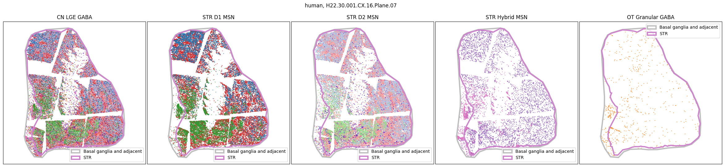
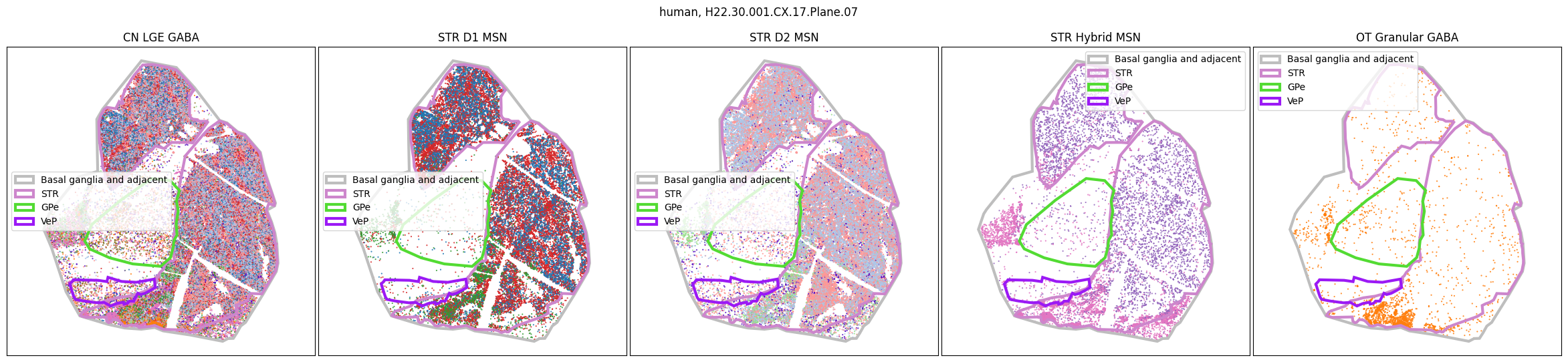
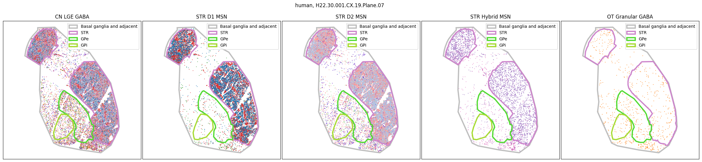
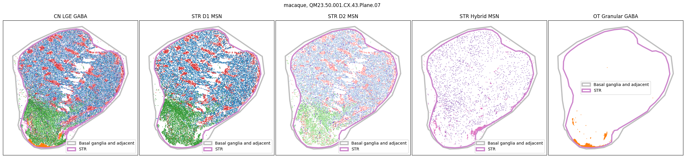
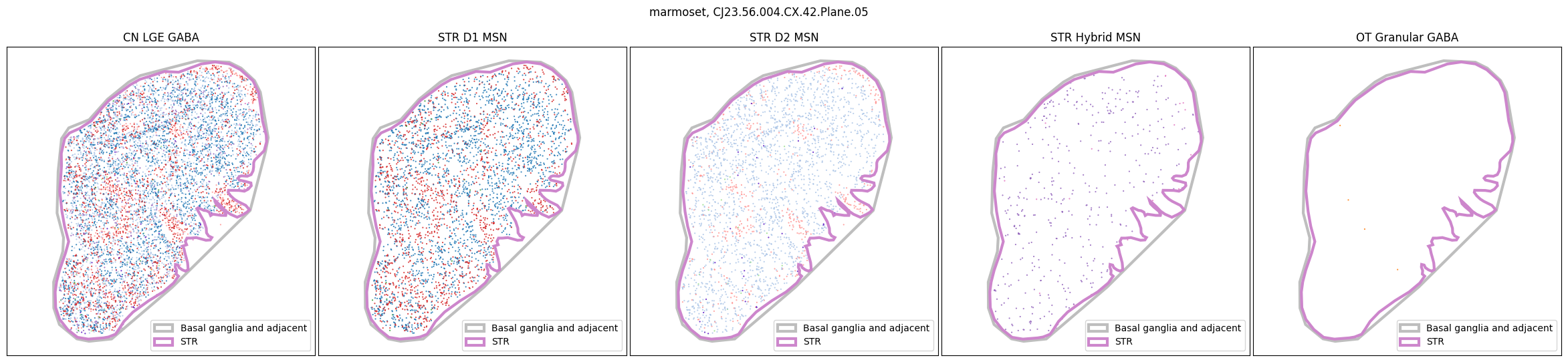
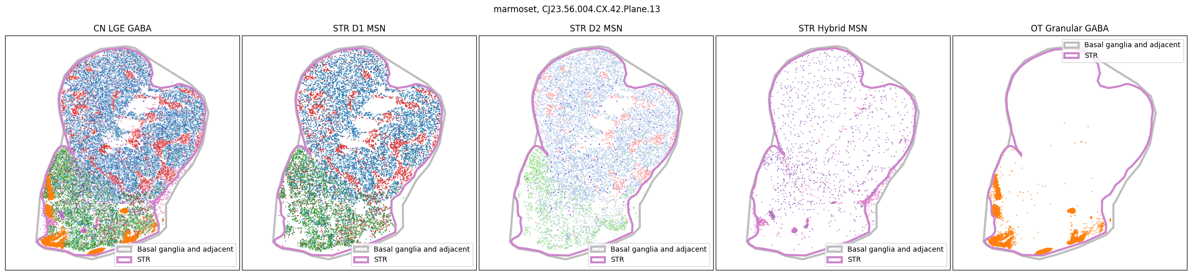
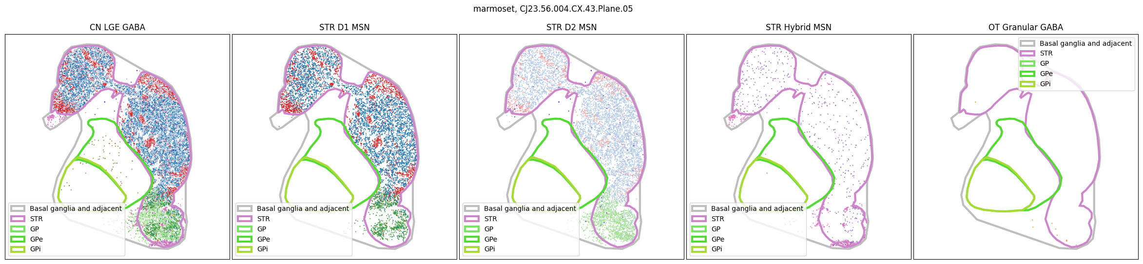
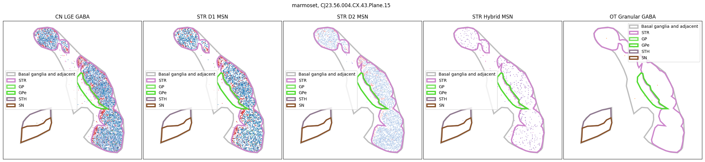
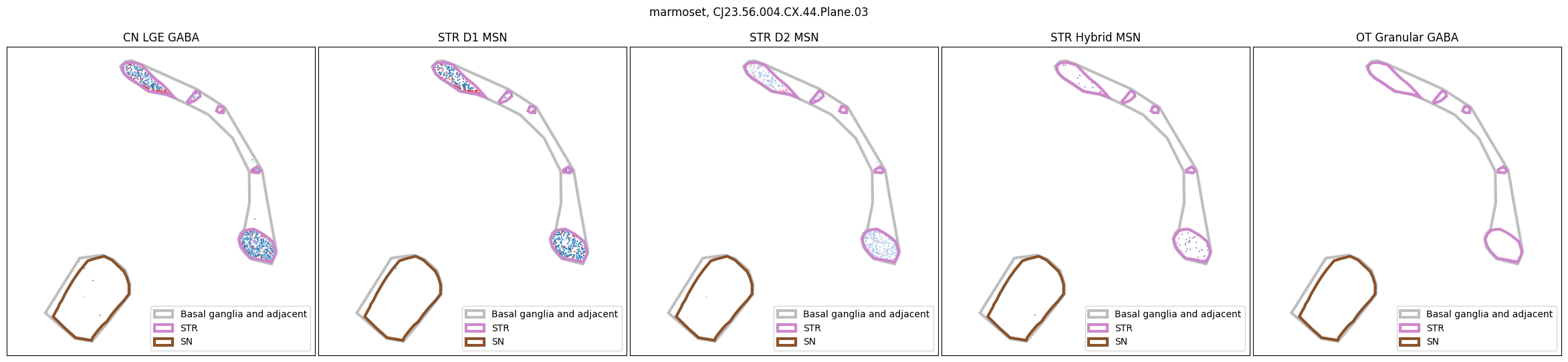
Selecting cell types

We define a slightly modified version of our slab plotting function that allows us to plot specific cell types, coloring by cell type level that is nominally lower in the taxonomy. This allows for us to investigate the spatial distribution of cell types more clearly by, for instance, plotting the spatial distributions of Groups within the a Medium Spiny Neuron subclass.

In general, cells associated with individual cell types and taxons can be selected by masking the DataFrame using the desired column and value in that column, as we showed in our examples above. For instance to select the Class, CN LGE GABA, we can create a mask thusly human_cell_metadata['Class']=='CN LGE GABA' and similarly for the other species. Again, this function can be used to plot individual slab planes and selections as well.

def plot_selected_cells(
    df: pd.DataFrame,
    feature: str,
    selection_list: List[Tuple[str, str]],
    slab: str,
    species: str,
    cmap: Optional[plt.Colormap] = None,
    fig_width: float = 40,
    fig_height: float = 8,
    plot_polygons: bool = True,
    point_size: float = 1.0,
    fix_bounds: bool = False
):
    """Plot spatial transcriptomics data selected a cell type and colored by
    a feature of interest.

    Parameters
    ----------
    df: pandas.DataFrame
        cell metadata data frame with x,y locations to plot.
    feature: str
        Expression value or color column to plot.
    selection_list: List[str]
        Set of cell types to select by. Specify as ('taxonomy_level_name', 'cell type')
    slab: str
        Specific slab to plot.
    species: str
        Species to plot (human, macaque, marmoset).
    cmap: matplotlib.colors.Colormap
        Colormap for expression features.
    fid_width: int
        Width of the plotted figure.
    fig_height: iont
        Height of the plotted figure.
    plot_polygons: bool
        Overplot geojson polygons. Note that these are note available for human
        and this should be set to False.
    point_size: float
        Size of the points to plot.
    fix_bounds: bool
        If True, fix the x and y bounds across all slabs to be the same.
    """
    
    fig, ax = plt.subplots(1, len(selection_list))
    fig.set_size_inches(fig_width, fig_height)

    if len(selection_list) == 1:
        ax = [ax]

    if 'slab_plane_label' in df.columns:
        slab_filtered = df[df['slab_plane_label']==slab]
    elif 'brain_section_label' in df.columns:
        slab_filtered = df[df['brain_section_label']==slab]

    if 'x' in df.columns:
        x_col = 'x'
    elif 'x_slab_mm' in df.columns:
        x_col = 'x_slab_mm'
    if 'y' in df.columns:
        y_col = 'y'
    elif 'y_slab_mm' in df.columns:
        y_col = 'y_slab_mm'

    if fix_bounds:
        x_min = slab_filtered[x_col].min()
        x_max = slab_filtered[x_col].max()
        y_min = slab_filtered[y_col].min()
        y_max = slab_filtered[y_col].max()
    
    for idx, (col, name) in enumerate(selection_list):

        if 'slab_plane_label' in df.columns:
            filtered = slab_filtered[slab_filtered[col]==name]
        elif 'brain_section_label' in df.columns:
            filtered = slab_filtered[slab_filtered[col]==name]
        xx = filtered[x_col]
        yy = filtered[y_col]
        vv = filtered[feature]
        
        if cmap is not None:
            ax[idx].scatter(xx, yy, s=point_size, c=vv, marker='.', cmap=cmap)
        else :
            ax[idx].scatter(xx, yy, s=point_size, c=vv, marker=".")

        if plot_polygons:
            plot_geo_data(get_polygons(slab, species=species), ax[idx])
            
        ax[idx].axis('equal')
        ylim = ax[idx].get_ylim()
        if fix_bounds:
            ylim = (y_min, y_max)
            ax[idx].set_xlim(x_min, x_max)
        ax[idx].set_ylim(ylim[1], ylim[0])
        ax[idx].set_xticks([])
        ax[idx].set_yticks([])
        
        ax[idx].set_title(name)
        ax[idx].legend(loc=0)
        
    plt.subplots_adjust(wspace=0.01, hspace=0.01)
    fig.suptitle(f'{species}, {slab}')
    return fig, ax

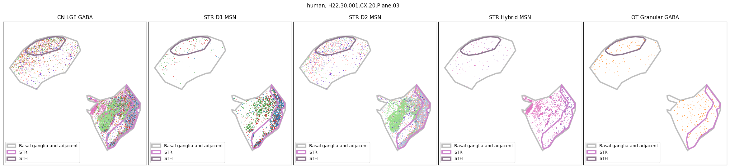
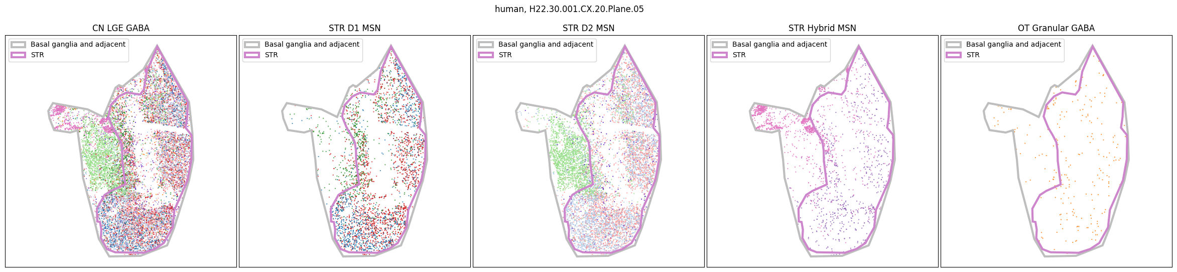
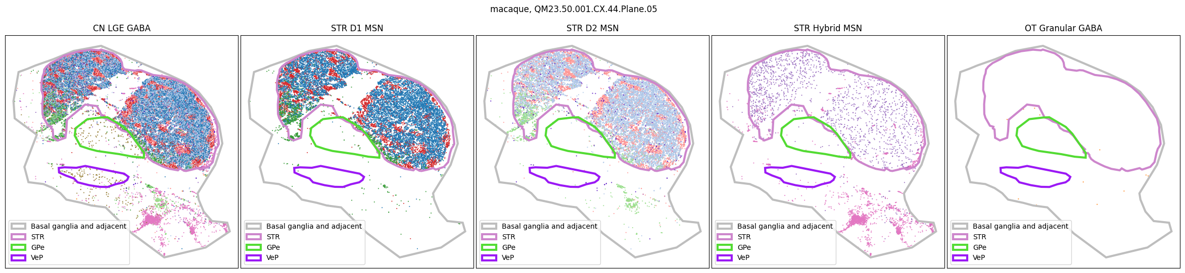
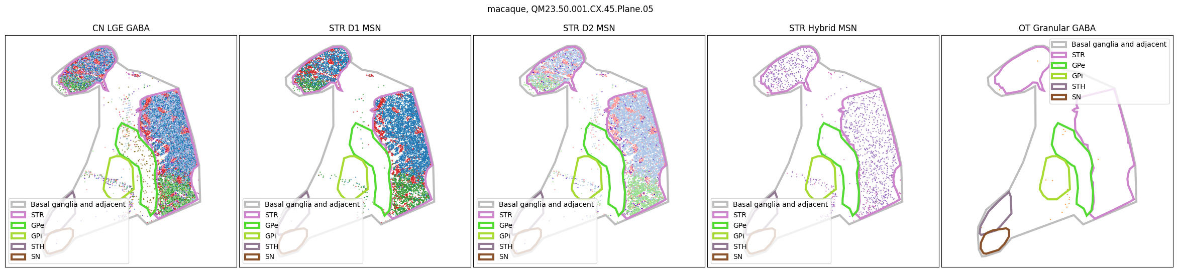
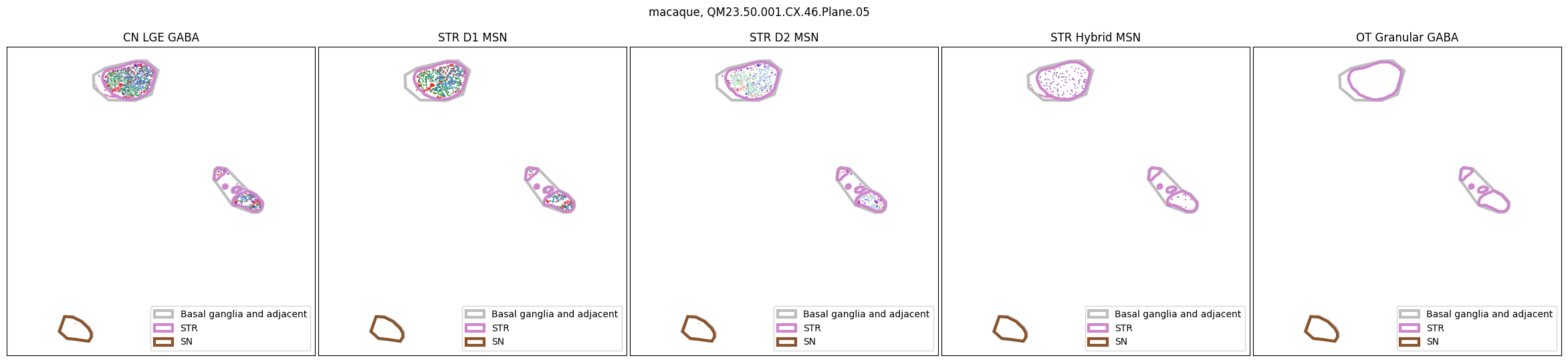
Using the above function, we plot the cells colored by their Group color and select by specific classes and subclasses. We can see commonalities in the distribution across the different species and sections,of the cell types exceptionally clearly.

for slab in human_slab_list:
    fig, ax = plot_selected_cells(
        human_cell_metadata,
        feature='Group_color',
        selection_list=[
            ('Class', 'CN LGE GABA'),
            ('Subclass', 'STR D1 MSN'),
            ('Subclass', 'STR D2 MSN'),
            ('Subclass', 'STR Hybrid MSN'),
            ('Subclass', 'OT Granular GABA')
        ],
        slab=slab,
        species='human',
        fig_width=30,
        fig_height=6,
        plot_polygons=True,
    )
    plt.show()

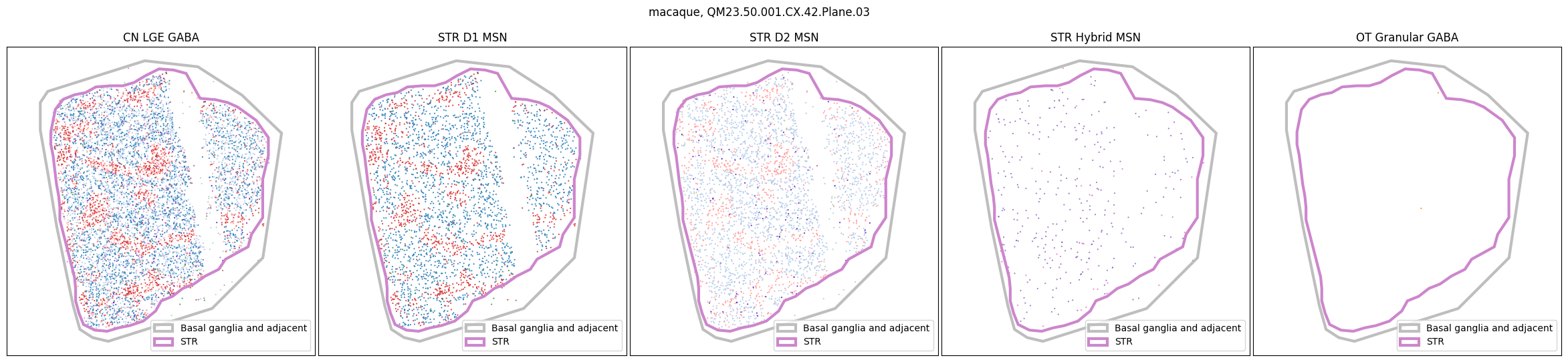
for slab in macaque_slab_list:
    fig, ax = plot_selected_cells(
        macaque_cell_metadata,
        feature='Group_color',
        selection_list=[
            ('Class', 'CN LGE GABA'),
            ('Subclass', 'STR D1 MSN'),
            ('Subclass', 'STR D2 MSN'),
            ('Subclass', 'STR Hybrid MSN'),
            ('Subclass', 'OT Granular GABA')
        ],
        slab=slab,
        species='macaque',
        fig_width=30,
        fig_height=6,
        plot_polygons=True,
    )

for slab in marmoset_slab_list:
    fig, ax = plot_selected_cells(
        marmoset_cell_metadata,
        feature='Group_color',
        selection_list=[
            ('Class', 'CN LGE GABA'),
            ('Subclass', 'STR D1 MSN'),
            ('Subclass', 'STR D2 MSN'),
            ('Subclass', 'STR Hybrid MSN'),
            ('Subclass', 'OT Granular GABA')
        ],
        slab=slab,
        species='marmoset',
        fig_width=30,
        fig_height=6,
        plot_polygons=True,
    )

In the next tutorial, we will explore gene expression patterns across these spatial transcriptomics datasets.

To learn more about the taxonomy used in this notebook and the data it is derived from, see the HMBA-BG Clustering Analysis and Taxonomy notebook.