Visualizing Neuronal Unit Responses

Note: Some of this content is adapted from the Allen SDK Documentation.

After processing Neuropixel ecephys data with Kilosort, individual neuronal units have been identified and are stored in the units table, in the Units section of the NWB file. The units table contains information about hypothetical neurons determined by Kilosort. With this information and the stimulus information found in the stimulus tables of the Intervals section, this notebook helps examine the spiking behavior of these units in response to stimulus and their associated waveforms

Environment Setup

⚠️Note: If running on a new environment, run this cell once and then restart the kernel⚠️

try:
    from databook_utils.dandi_utils import dandi_download_open
except:
    !git clone https://github.com/AllenInstitute/openscope_databook.git
    %cd openscope_databook
    %pip install -e .

import matplotlib as mpl
import matplotlib.pyplot as plt
import numpy as np

%matplotlib inline

Downloading Ecephys File

Change the values below to download the file you’re interested in. Set dandiset_id and dandi_filepath to correspond to the dandiset id and filepath of the file you want. If you’re accessing an embargoed dataset, set dandi_api_key to your DANDI API key. If you want to stream a file instead of downloading it, use dandi_stream_open instead. Checkout Streaming an NWB File with fsspec for more details on this.

dandiset_id = "000021"
dandi_filepath = "sub-703279277/sub-703279277_ses-719161530.nwb"
download_loc = "."
dandi_api_key = None

# This can sometimes take a while depending on the size of the file
io = dandi_download_open(dandiset_id, dandi_filepath, download_loc, dandi_api_key=dandi_api_key)
nwb = io.read()

File already exists
Opening file

c:\Users\carter.peene\AppData\Local\Programs\Python\Python39\lib\site-packages\hdmf\spec\namespace.py:531: UserWarning: Ignoring cached namespace 'hdmf-common' version 1.1.3 because version 1.5.1 is already loaded.
  warn("Ignoring cached namespace '%s' version %s because version %s is already loaded."
c:\Users\carter.peene\AppData\Local\Programs\Python\Python39\lib\site-packages\hdmf\spec\namespace.py:531: UserWarning: Ignoring cached namespace 'core' version 2.2.2 because version 2.5.0 is already loaded.
  warn("Ignoring cached namespace '%s' version %s because version %s is already loaded."

Extracting Unit Data and Stimulus Data

Below, the Units table is read from the file. Individual units (putative neurons) are identified with the id column. Note that, while each id is unique, they are not perfectly ordinal; some ids are missing. In the cells below, the unit properties are listed and a slice of the units table is shown. More thorough descriptions of units and their properties can be found in Visualizing Unit Quality Metrics

Additionally, the stimulus data is also read from the NWB file’s Intervals section. Stimulus information is stored as a series of tables depending on the type of stimulus shown in the session. One such table is displayed below.

units = nwb.units
units.colnames

('waveform_duration',
 'cluster_id',
 'peak_channel_id',
 'cumulative_drift',
 'amplitude_cutoff',
 'snr',
 'recovery_slope',
 'isolation_distance',
 'nn_miss_rate',
 'silhouette_score',
 'velocity_above',
 'quality',
 'PT_ratio',
 'l_ratio',
 'velocity_below',
 'max_drift',
 'isi_violations',
 'firing_rate',
 'amplitude',
 'local_index',
 'spread',
 'waveform_halfwidth',
 'd_prime',
 'presence_ratio',
 'repolarization_slope',
 'nn_hit_rate',
 'spike_times',
 'spike_amplitudes',
 'waveform_mean')

units[:10]

	waveform_duration	cluster_id	peak_channel_id	cumulative_drift	amplitude_cutoff	snr	recovery_slope	isolation_distance	nn_miss_rate	silhouette_score	...	local_index	spread	waveform_halfwidth	d_prime	presence_ratio	repolarization_slope	nn_hit_rate	spike_times	spike_amplitudes	waveform_mean
id
950921187	0.604355	4	850249267	481.80	0.425574	2.209140	-0.118430	17.537571	0.009496	0.036369	...	4	50.0	0.357119	2.962274	0.99	0.381716	0.473829	[1.0439430431793884, 1.543311060144649, 2.7287...	[0.0001908626967721937, 0.00016134635752077775...	[[0.0, 0.5961149999999966, 5.378099999999993, ...
950921172	0.521943	3	850249267	681.53	0.390098	1.959983	-0.109729	14.677643	0.003857	0.103446	...	3	40.0	0.260972	2.067810	0.99	0.536663	0.445946	[10.406435026164546, 17.127986534673788, 18.48...	[0.00014485615850768024, 0.0001722424107984555...	[[0.0, -1.341600000000002, -0.4586399999999933...
950921152	0.467002	2	850249267	1070.71	0.500000	2.522905	-0.109867	15.783665	0.017776	0.027818	...	2	50.0	0.247236	2.220043	0.99	0.566559	0.284058	[1.2775103414155262, 2.3915133536963493, 3.701...	[0.00014859435856024575, 0.0001531048673600236...	[[0.0, -0.6427199999999993, -2.836079999999998...
950921135	0.467002	1	850249267	253.42	0.500000	2.803475	-0.150379	26.666930	0.023742	0.076530	...	1	40.0	0.233501	2.339206	0.99	0.669090	0.590737	[9.473732504122962, 13.198542576065163, 18.302...	[0.00032386170367170055, 0.0004518112387675137...	[[0.0, -3.2800950000000078, -6.087510000000009...
950921111	0.439531	0	850249267	141.82	0.018056	4.647943	-0.328727	66.901065	0.006595	NaN	...	0	30.0	0.219765	4.395994	0.99	1.261416	0.952667	[1.1677100445138795, 1.1707767194728813, 1.349...	[0.00015644521007973124, 0.000214412247939483,...	[[0.0, -0.9291749999999945, -6.120270000000007...
950927711	1.455946	482	850249273	2.46	0.000895	1.651500	-0.039932	39.400278	0.000033	NaN	...	464	100.0	0.274707	5.557479	0.37	0.467365	0.000000	[2613.8652081509977, 2624.5193369599215, 2734....	[0.00012946663895843286, 0.0001203425053985725...	[[0.0, 6.3216435986159105, 10.324204152249129,...
950921285	2.087772	11	850249273	318.53	0.036848	1.379817	NaN	27.472722	0.000903	0.291953	...	11	100.0	0.288442	2.751337	0.89	0.372116	0.258065	[39.04904580954626, 39.457346913598556, 40.495...	[7.768399792002802e-05, 8.405736507197006e-05,...	[[0.0, 5.330324999999991, 2.4261899999999486, ...
950921271	0.947739	10	850249273	1008.50	0.001727	1.420617	-0.008204	30.027595	0.000707	0.406673	...	10	100.0	0.288442	3.847234	0.96	0.498618	0.796491	[16.751918851114475, 26.127977537450867, 28.65...	[0.00016516929470324686, 0.0001501058102103845...	[[0.0, -3.103230000000032, 5.680349999999983, ...
950921260	0.453266	9	850249273	175.00	0.000081	4.969091	-0.184456	89.804006	0.000000	0.223876	...	9	60.0	0.192295	5.274090	0.99	1.140487	0.997333	[0.9620761551434307, 2.092045877265143, 2.4040...	[0.0003836112198262231, 0.0004093908262843732,...	[[0.0, 1.9104149999999982, -7.270770000000016,...
950921248	0.439531	8	850249273	261.11	0.065478	2.147758	-0.085677	84.145512	0.005474	0.076346	...	8	60.0	0.274707	3.022387	0.99	0.463570	0.976667	[1.316477113448928, 1.779311698293908, 2.96088...	[0.00013780619334124896, 0.0001439873831056905...	[[0.0, -3.6761399999999953, 0.8334300000000014...

10 rows × 29 columns

stimulus_names = nwb.intervals.keys()
print(stimulus_names)

dict_keys(['drifting_gratings_presentations', 'flashes_presentations', 'gabors_presentations', 'invalid_times', 'natural_movie_one_presentations', 'natural_movie_three_presentations', 'natural_scenes_presentations', 'spontaneous_presentations', 'static_gratings_presentations'])

stim_table = nwb.intervals["flashes_presentations"]
stim_table[:]

	start_time	stop_time	stimulus_name	stimulus_block	color	mask	opacity	phase	size	units	stimulus_index	orientation	spatial_frequency	contrast	tags	timeseries
id
0	1290.883097	1291.133309	flashes	1.0	-1.0	None	1.0	[0.0, 0.0]	[300.0, 300.0]	deg	1.0	0.0	[0.0, 0.0]	0.8	[stimulus_time_interval]	[(3647, 1, timestamps pynwb.base.TimeSeries at...
1	1292.884817	1293.135016	flashes	1.0	1.0	None	1.0	[0.0, 0.0]	[300.0, 300.0]	deg	1.0	0.0	[0.0, 0.0]	0.8	[stimulus_time_interval]	[(3648, 1, timestamps pynwb.base.TimeSeries at...
2	1294.886487	1295.136691	flashes	1.0	1.0	None	1.0	[0.0, 0.0]	[300.0, 300.0]	deg	1.0	0.0	[0.0, 0.0]	0.8	[stimulus_time_interval]	[(3649, 1, timestamps pynwb.base.TimeSeries at...
3	1296.888137	1297.138344	flashes	1.0	1.0	None	1.0	[0.0, 0.0]	[300.0, 300.0]	deg	1.0	0.0	[0.0, 0.0]	0.8	[stimulus_time_interval]	[(3650, 1, timestamps pynwb.base.TimeSeries at...
4	1298.889787	1299.140004	flashes	1.0	-1.0	None	1.0	[0.0, 0.0]	[300.0, 300.0]	deg	1.0	0.0	[0.0, 0.0]	0.8	[stimulus_time_interval]	[(3651, 1, timestamps pynwb.base.TimeSeries at...
...	...	...	...	...	...	...	...	...	...	...	...	...	...	...	...	...
145	1581.125517	1581.375726	flashes	1.0	1.0	None	1.0	[0.0, 0.0]	[300.0, 300.0]	deg	1.0	0.0	[0.0, 0.0]	0.8	[stimulus_time_interval]	[(3792, 1, timestamps pynwb.base.TimeSeries at...
146	1583.127217	1583.377419	flashes	1.0	1.0	None	1.0	[0.0, 0.0]	[300.0, 300.0]	deg	1.0	0.0	[0.0, 0.0]	0.8	[stimulus_time_interval]	[(3793, 1, timestamps pynwb.base.TimeSeries at...
147	1585.128807	1585.379029	flashes	1.0	-1.0	None	1.0	[0.0, 0.0]	[300.0, 300.0]	deg	1.0	0.0	[0.0, 0.0]	0.8	[stimulus_time_interval]	[(3794, 1, timestamps pynwb.base.TimeSeries at...
148	1587.130507	1587.380724	flashes	1.0	-1.0	None	1.0	[0.0, 0.0]	[300.0, 300.0]	deg	1.0	0.0	[0.0, 0.0]	0.8	[stimulus_time_interval]	[(3795, 1, timestamps pynwb.base.TimeSeries at...
149	1589.132187	1589.382401	flashes	1.0	-1.0	None	1.0	[0.0, 0.0]	[300.0, 300.0]	deg	1.0	0.0	[0.0, 0.0]	0.8	[stimulus_time_interval]	[(3796, 1, timestamps pynwb.base.TimeSeries at...

150 rows × 16 columns

Getting Stimulus Epochs

Here, epochs are extracted from the stimulus tables. In this case, an epoch is a continuous period of time during a session where a particular type of stimulus is shown. The output here is a list of epochs, where an epoch is a tuple of four values; the stimulus name, the stimulus block, the starting time and the ending time. Since stimulus information can vary significantly between experiments and NWB files, you may need to tailor the code below to extract epochs for the file you’re interested in.

# extract epoch times from stim table where stimulus rows have a different 'block' than following row
# returns list of epochs, where an epoch is of the form (stimulus name, stimulus block, start time, stop time)
def extract_epochs(stim_name, stim_table, epochs):
    
    # specify a current epoch stop and start time
    epoch_start = stim_table.start_time[0]
    epoch_stop = stim_table.stop_time[0]

    # for each row, try to extend current epoch stop_time
    for i in range(len(stim_table)):
        this_block = stim_table.stimulus_block[i]
        # if end of table, end the current epoch
        if i+1 >= len(stim_table):
            epochs.append((stim_name, this_block, epoch_start, epoch_stop))
            break
            
        next_block = stim_table.stimulus_block[i+1]
        # if next row is the same stim block, push back epoch_stop time
        if next_block == this_block:
            epoch_stop = stim_table.stop_time[i+1]
        # otherwise, end the current epoch, start new epoch
        else:
            epochs.append((stim_name, this_block, epoch_start, epoch_stop))
            epoch_start = stim_table.start_time[i+1]
            epoch_stop = stim_table.stop_time[i+1]
    
    return epochs

# extract epochs from all valid stimulus tables
epochs = []
for stim_name in stimulus_names:
    stim_table = nwb.intervals[stim_name]
    try:
        epochs = extract_epochs(stim_name, stim_table, epochs)
    except:
        continue

# epochs take the form (stimulus name, stimulus block, start time, stop time)
print(len(epochs))
epochs.sort(key=lambda x: x[2])
for epoch in epochs:
    print(epoch)

15
('gabors_presentations', 0.0, 89.8968273815905, 1001.8917716749913)
('flashes_presentations', 1.0, 1290.8830973815907, 1589.382401312724)
('drifting_gratings_presentations', 2.0, 1591.1338573815906, 2190.634543106125)
('natural_movie_three_presentations', 3.0, 2221.6604473815905, 2822.161967381591)
('natural_movie_one_presentations', 4.0, 2852.1870373815905, 3152.4377773815904)
('drifting_gratings_presentations', 5.0, 3182.4628573815908, 3781.963503106125)
('natural_movie_three_presentations', 6.0, 4083.215117381591, 4683.716567381592)
('drifting_gratings_presentations', 7.0, 4713.741627381592, 5397.312443106124)
('static_gratings_presentations', 8.0, 5398.31325738159, 5878.714467381591)
('natural_scenes_presentations', 9.0, 5908.739537381591, 6389.157337381589)
('natural_scenes_presentations', 10.0, 6689.408117381589, 7169.809297381591)
('static_gratings_presentations', 11.0, 7199.83431738159, 7680.268867381591)
('natural_movie_one_presentations', 12.0, 7710.293937381591, 8010.54467738159)
('natural_scenes_presentations', 13.0, 8040.56972738159, 8568.510620243858)
('static_gratings_presentations', 14.0, 8611.04613738159, 9151.49746738159)

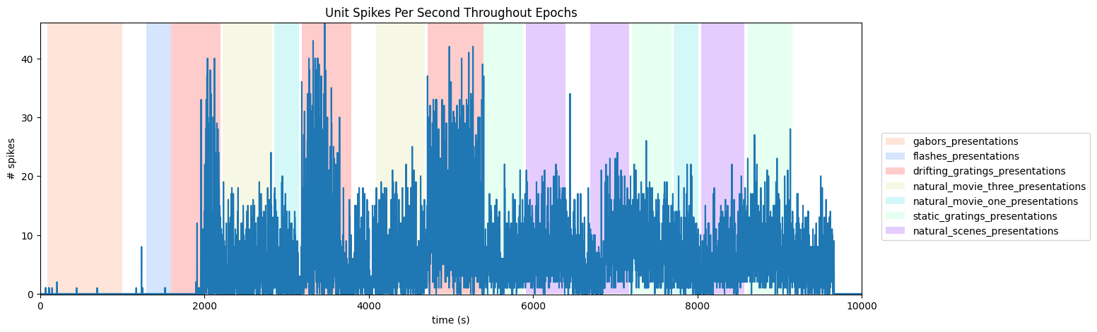
Visualizing Unit Activity Throughout Epochs

Below is a view of the spiking activity of a unit throughout a session, where epochs are shown as colored sections. Set unit_num to be the id of the unit to view. Set time_start to the starting bound in seconds of the session, you’d like to see, and time_end to the ending bound. You may want to use the output above to inform your choice. As mentioned above, if your file’s stimulus information differs significantly, this code may need to be modified to appropriately display the epochs.

unit_num = 950930672 # chosen from units table
time_start = 0
time_end = 10000

# translate unit id to row index
unit_idx = -1
for i in range(len(units.id)):
    if units.id[i] == unit_num:
        unit_idx = i
        break
print("Unit index:",unit_idx)

Unit index: 648

# make histogram of unit spikes per second over specified timeframe
spikes = units["spike_times"][unit_idx]
time_bin_edges = np.linspace(time_start, time_end, (time_end-time_start))
hist, bins = np.histogram(spikes, bins=time_bin_edges)

# generate plot of spike histogram with colored epoch intervals and legend
fig, ax = plt.subplots(figsize=(15,5))

# assign unique color to each stimulus name
stim_names = list({epoch[0] for epoch in epochs})
colors = plt.cm.rainbow(np.linspace(0,1,len(stim_names)))
stim_color_map = {stim_names[i]:colors[i] for i in range(len(stim_names))}

epoch_key = {}
height = max(hist)
# draw colored rectangles for each epoch
for epoch in epochs:
    stim_name, stim_block, epoch_start, epoch_end = epoch
    color = stim_color_map[stim_name]
    rec = ax.add_patch(mpl.patches.Rectangle((epoch_start, 0), epoch_end-epoch_start, height, alpha=0.2, facecolor=color))
    epoch_key[stim_name] = rec
    
ax.set_xlim(time_start, time_end)
ax.set_ylim(-0.1, height+0.1)
ax.set_xlabel("time (s)")
ax.set_ylabel("# spikes")
ax.set_title("Unit Spikes Per Second Throughout Epochs")

fig.legend(epoch_key.values(), epoch_key.keys(), loc="lower right", bbox_to_anchor=(1.12, 0.25))
ax.plot(bins[:-1], hist)

[<matplotlib.lines.Line2D at 0x21ca7568760>]

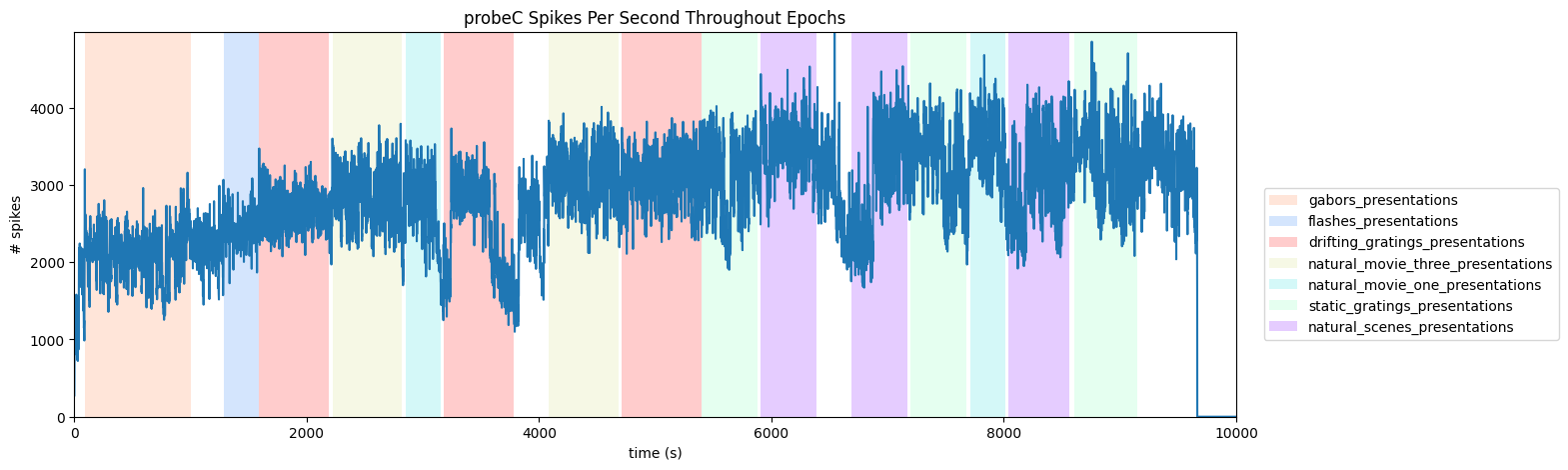
Probewise Activity Throughout Epochs

It can also be useful to view the activity of an entire probe throughout epochs. The code below allows users to select a probe and a histogram is produced for the total of all unit spiking counts over time for one probe. To do this, the file’s Electrodes table is used. To understand this, you need not know anything about the Electrodes table, except that it can be used to map channel IDs to probe IDs. Below is printed a list of the probe names to choose from. Set probe_name to one of these. Set time_start and time_end to the start and ending times, in seconds, to view in the session.

print(nwb.devices.keys())

dict_keys(['probeA', 'probeB', 'probeC', 'probeD', 'probeE', 'probeF'])

probe_name = "probeC"
time_start = 0
time_end = 10000

# get list of channels on this probe
electrodes = nwb.electrodes.to_dataframe()
channel_ids = set(electrodes.index[electrodes["group_name"] == probe_name].tolist())

# get all spike times from units whose peak channel belongs to the selected probe
probe_spike_times = []
for i in range(len(units)):
    if units["peak_channel_id"][i] in channel_ids:
        probe_spike_times += list(units["spike_times"][i])
    
len(probe_spike_times)

27741944

# make histogram of unit spikes per second over specified timeframe
time_bin_edges = np.linspace(time_start, time_end, (time_end-time_start))
hist, bins = np.histogram(probe_spike_times, bins=time_bin_edges)

# generate plot of spike histogram with colored epoch intervals and legend
fig, ax = plt.subplots(figsize=(15,5))

# assign unique color to each stimulus name
stim_names = list({epoch[0] for epoch in epochs})
colors = plt.cm.rainbow(np.linspace(0,1,len(stim_names)))
stim_color_map = {stim_names[i]:colors[i] for i in range(len(stim_names))}

epoch_key = {}
height = max(hist)
# draw colored rectangles for each epoch
for epoch in epochs:
    stim_name, stim_block, epoch_start, epoch_end = epoch
    color = stim_color_map[stim_name]
    rec = ax.add_patch(mpl.patches.Rectangle((epoch_start, 0), epoch_end-epoch_start, height, alpha=0.2, facecolor=color))
    epoch_key[stim_name] = rec
    
ax.set_xlim(time_start, time_end)
ax.set_ylim(-0.1, height+0.1)
ax.set_xlabel("time (s)")
ax.set_ylabel("# spikes")
ax.set_title(f"{probe_name} Spikes Per Second Throughout Epochs")

fig.legend(epoch_key.values(), epoch_key.keys(), loc="lower right", bbox_to_anchor=(1.12, 0.25))
ax.plot(bins[:-1], hist)

[<matplotlib.lines.Line2D at 0x21d04bdc610>]

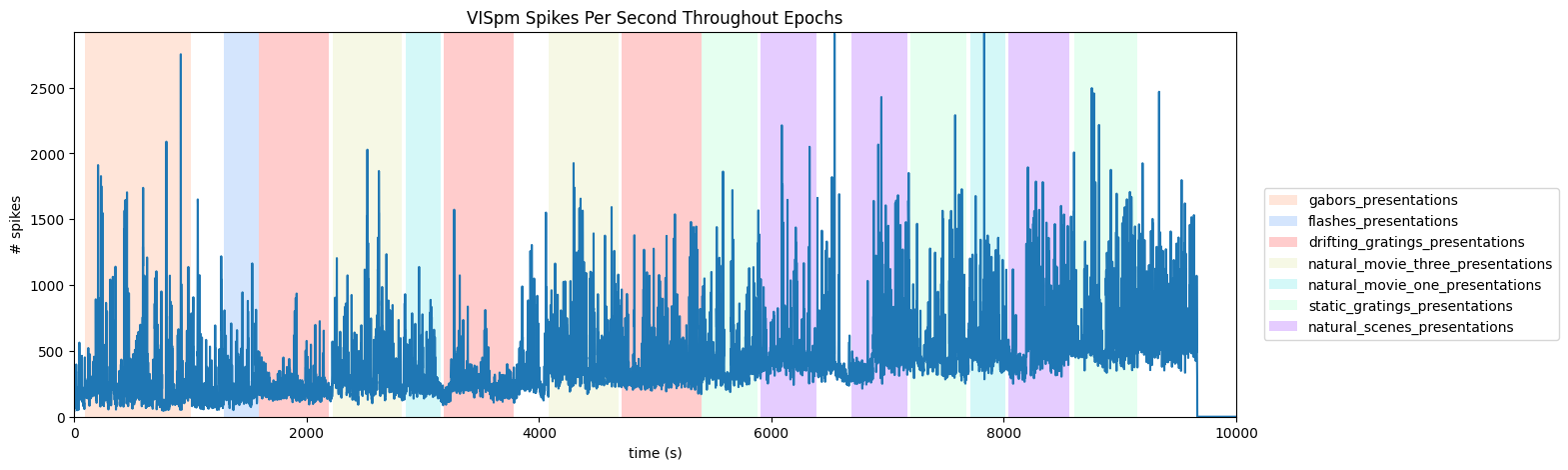
Regionwise Activity Throughout Epochs

We can also break down our activity based on brain regions (with a bit of work). To do this, we must first be able to retrieve the brain region of each unit. The trick to do this lay in the Electrodes table, shown below. The Electrodes table contains the brain region for each electrode id, while the Units table (shown above) contains the Peak Channel ID for each Unit. These can be used together to get the brain region of each unit’s peak channel. Once this is done, this information can be used just like the Probe selection above to get to get spike counts over time of each Unit in a selected region. Below, set brain_region, start_time, and end_time to view such a plot.

nwb.electrodes[:10]

	x	y	z	imp	location	filtering	group	group_name	probe_vertical_position	probe_horizontal_position	probe_id	local_index	valid_data
id
850249265	7955.0	3766.0	3766.0	NaN	Eth	AP band: 500 Hz high-pass; LFP band: 1000 Hz l...	probeB abc.EcephysElectrodeGroup at 0x23221155...	probeB	20	43	729445650	0	False
850249267	7955.0	3756.0	3756.0	NaN	TH	AP band: 500 Hz high-pass; LFP band: 1000 Hz l...	probeB abc.EcephysElectrodeGroup at 0x23221155...	probeB	20	11	729445650	1	True
850249273	7955.0	3727.0	3727.0	NaN	TH	AP band: 500 Hz high-pass; LFP band: 1000 Hz l...	probeB abc.EcephysElectrodeGroup at 0x23221155...	probeB	60	43	729445650	4	True
850249277	7954.0	3708.0	3708.0	NaN	APN	AP band: 500 Hz high-pass; LFP band: 1000 Hz l...	probeB abc.EcephysElectrodeGroup at 0x23221155...	probeB	80	59	729445650	6	True
850249283	7954.0	3679.0	3679.0	NaN	APN	AP band: 500 Hz high-pass; LFP band: 1000 Hz l...	probeB abc.EcephysElectrodeGroup at 0x23221155...	probeB	100	11	729445650	9	True
850249289	7953.0	3640.0	3640.0	NaN	APN	AP band: 500 Hz high-pass; LFP band: 1000 Hz l...	probeB abc.EcephysElectrodeGroup at 0x23221155...	probeB	140	43	729445650	12	True
850249295	7952.0	3612.0	3612.0	NaN	APN	AP band: 500 Hz high-pass; LFP band: 1000 Hz l...	probeB abc.EcephysElectrodeGroup at 0x23221155...	probeB	160	27	729445650	15	True
850249299	7952.0	3593.0	3593.0	NaN	APN	AP band: 500 Hz high-pass; LFP band: 1000 Hz l...	probeB abc.EcephysElectrodeGroup at 0x23221155...	probeB	180	11	729445650	17	True
850249305	7951.0	3565.0	3565.0	NaN	APN	AP band: 500 Hz high-pass; LFP band: 1000 Hz l...	probeB abc.EcephysElectrodeGroup at 0x23221155...	probeB	220	43	729445650	20	True
850249311	7950.0	3537.0	3537.0	NaN	APN	AP band: 500 Hz high-pass; LFP band: 1000 Hz l...	probeB abc.EcephysElectrodeGroup at 0x23221155...	probeB	240	27	729445650	23	True

# map electrode ids to brain region acronyms
electrode_locations = {nwb.electrodes["id"][i]: nwb.electrodes["location"][i] for i in range(len(nwb.electrodes))}
print(set(electrode_locations.values()))

{'', 'VISpm', 'CA2', 'NOT', 'VISp', 'Eth', 'VISal', 'VISrl', 'MB', 'DG', 'VPM', 'CA3', 'PO', 'APN', 'LP', 'VISl', 'grey', 'TH', 'SUB', 'LGd', 'VISam', 'POL', 'CA1', 'VL'}

brain_region = "VISpm"
time_start = 0
time_end = 10000

# get all spike times from units whose peak channel belongs to the selected brain region
region_spike_times = []
for i in range(len(units)):
    unit_channel = units["peak_channel_id"][i]
    unit_location = electrode_locations.get(unit_channel, None)
    if unit_location == brain_region:
        region_spike_times += list(units["spike_times"][i])
    
len(region_spike_times)

4178172

# make histogram of unit spikes per second over specified timeframe
time_bin_edges = np.linspace(time_start, time_end, (time_end-time_start))
hist, bins = np.histogram(region_spike_times, bins=time_bin_edges)

# generate plot of spike histogram with colored epoch intervals and legend
fig, ax = plt.subplots(figsize=(15,5))

# assign unique color to each stimulus name
stim_names = list({epoch[0] for epoch in epochs})
colors = plt.cm.rainbow(np.linspace(0,1,len(stim_names)))
stim_color_map = {stim_names[i]:colors[i] for i in range(len(stim_names))}

epoch_key = {}
height = max(hist)
# draw colored rectangles for each epoch
for epoch in epochs:
    stim_name, stim_block, epoch_start, epoch_end = epoch
    color = stim_color_map[stim_name]
    rec = ax.add_patch(mpl.patches.Rectangle((epoch_start, 0), epoch_end-epoch_start, height, alpha=0.2, facecolor=color))
    epoch_key[stim_name] = rec
    
ax.set_xlim(time_start, time_end)
ax.set_ylim(-0.1, height+0.1)
ax.set_xlabel("time (s)")
ax.set_ylabel("# spikes")
ax.set_title(f"{brain_region} Spikes Per Second Throughout Epochs")

fig.legend(epoch_key.values(), epoch_key.keys(), loc="lower right", bbox_to_anchor=(1.12, 0.25))
ax.plot(bins[:-1], hist)

[<matplotlib.lines.Line2D at 0x21d0c9b2760>]

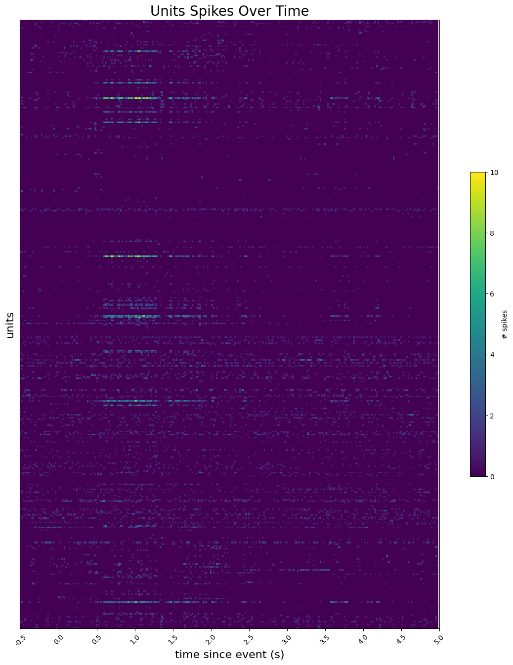
Showing Spike Times

Here, a histogram plot of unit spikes over time is created. In the second cell below, set stim_time to be the time of the stimulus you’re interested in viewing. To get an idea of the stimulus times you might be interested in, access one of the tables in the Intervals section, discussed above in Extracting Unit Data and Stimulus Data. The first cell below shows how to access these. Set interval_start and interval_end to the relative time bounds, in seconds, of the histogram around stim_time. Finally, start_unit and end_unit can be used to choose the slice indices of selected_units to display.

stim_time = 1007 # arbitrarily chosen here
interval_start = -0.1
interval_end = 5

start_unit = 100
end_unit = 500

spike_times = [elem for elem in units["spike_times"][start_unit:end_unit]]
if len(spike_times) == 0:
    raise Exception("There are no spiking units in this selection")
len(spike_times)

400

# for each unit, generate a histogram with 200 bins, where bins represent the number spikes per second
time_bin_edges = np.linspace(interval_start, interval_end, 200)
hists = []
for unit_spike_times in spike_times:
    hist, bins = np.histogram(unit_spike_times-stim_time, bins=time_bin_edges)
    hists.append(hist)
hists = np.array(hists)

hists.shape

(400, 199)

# display array of histograms as 2D image with color
fig, ax = plt.subplots(figsize=(16,16))
img = ax.imshow(hists)
cbar = plt.colorbar(img, shrink=0.5)
cbar.set_label('# spikes')

ax.yaxis.set_major_locator(plt.NullLocator())
ax.set_ylabel("units", fontsize=16)

xtick_step=20
reltime = np.array(time_bin_edges)
ax.set_xticks(np.arange(0, len(reltime), xtick_step))
ax.set_xticklabels([f'{mp:1.3f}' for mp in reltime[::xtick_step]], rotation=45)

ax.set_xlabel("time since event (s)", fontsize=16)
ax.set_title("Units Spikes Over Time", fontsize=20)

Text(0.5, 1.0, 'Units Spikes Over Time')

Visualizing Waveforms

The Units table can also be used to view the waveforms of a units with the waveform_mean property, which consists of the mean waveform of that unit as measured by each channel along the probe. One channel will contain the peak waveform. With a bit of legwork, the peak_channel_id of the unit and the Electrodes table can be used to get the single peak waveform as shown below. Just as in the sections above, you don’t need to fully understand the Electrodes table except that it can be used to map channel IDs to probe IDs. There is also a timewise and channelwise view of all the mean waveforms and an average of the waveforms across all channels.

unit_num = 950952910

# translate unit id to row index
unit_idx = -1
for i in range(len(units.id)):
    if units.id[i] == unit_num:
        unit_idx = i
        break
print("Unit index:",unit_idx)

Unit index: 2513

# get sampling Hz for this unit's waveform
peak_channel_id = units["peak_channel_id"][unit_idx]
electrodes = nwb.electrodes.to_dataframe()
probe_name = electrodes.loc[peak_channel_id].group_name

Hz = nwb.devices[probe_name].sampling_rate
Hz

29999.9995000281

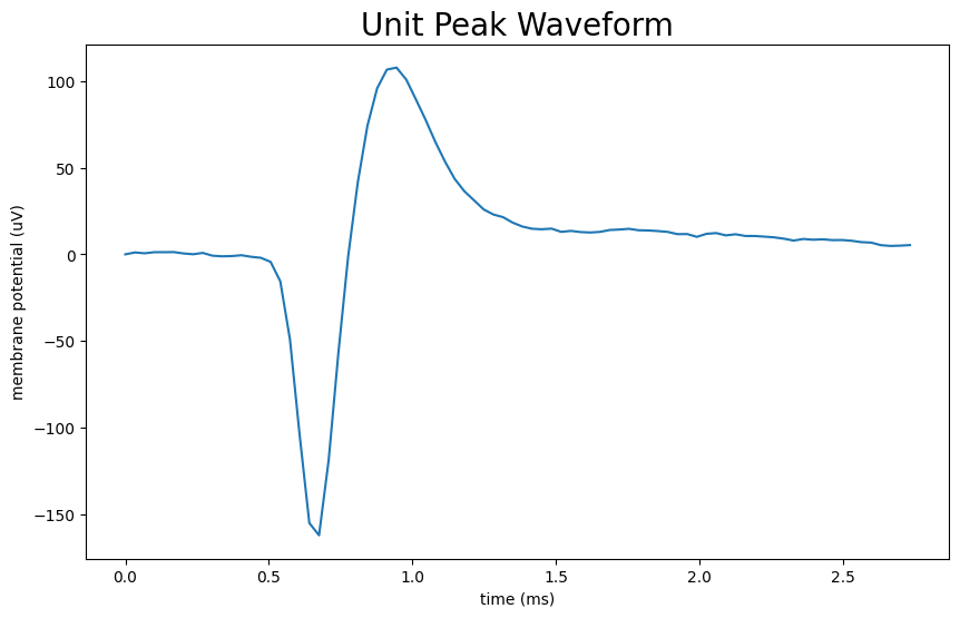
Peak waveform

# use peak_channel_id of unit to fetch the peak waveform index from electrodes table
peak_channel_id = units["peak_channel_id"][unit_idx]
electrodes = nwb.electrodes.to_dataframe()
local_index = electrodes.loc[peak_channel_id].local_index

unit_waveform = units["waveform_mean"][unit_idx]
peak_waveform = unit_waveform[local_index]

fig, ax = plt.subplots(figsize=(10,6))

n_secs = peak_waveform.shape[0] / Hz
time_axis = np.linspace(0, n_secs * 1000, peak_waveform.shape[0])

ax.plot(time_axis, peak_waveform)

ax.set_xlabel("time (ms)")
ax.set_ylabel("membrane potential (uV)")
ax.set_title("Unit Peak Waveform", fontsize=20)

plt.show()

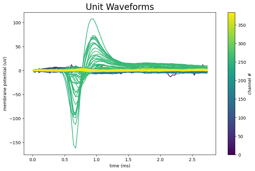
Waveforms

unit_waveforms = units["waveform_mean"][unit_idx]
unit_waveforms.shape

(384, 82)

fig, ax = plt.subplots(figsize=(10,6))
colors = plt.cm.viridis(np.linspace(0, 1, unit_waveforms.shape[0]))
ax.set_prop_cycle(color=colors)

n_secs = unit_waveforms.shape[1] / Hz
time_axis = np.linspace(0, n_secs * 1000, unit_waveforms.shape[1])

ax.plot(time_axis, np.transpose(unit_waveforms))

norm = mpl.colors.Normalize(vmin=0, vmax=len(colors))
cb = fig.colorbar(mpl.cm.ScalarMappable(norm=norm), ax=ax, label='channel #')

ax.set_xlabel("time (ms)")
ax.set_ylabel("membrane potential (uV)")
ax.set_title("Unit Waveforms", fontsize=20)

plt.show()

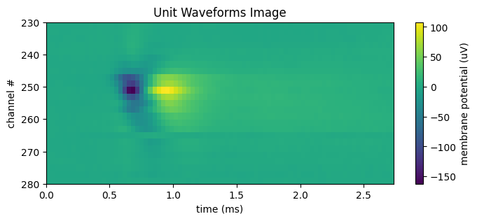
Waveform Image

Below is an image of the waveform means for each channel of a unit. The further in space from the real neuron, the weaker the measurement of the response waveform, so it is usually only useful to view a subsection of the channels at once. Set start_channel and end_channel to be the bounds of the channels you want displayed. Because the channels are arranged into two rows along the length of a probe, typically a unit is only strongly detected by every other channel. The data shown below displays every other channel to avoid the resultant striping effect. If the waveform looks too dim, try incrementing start_channel by 1.

start_channel = 230
end_channel = 280

data = unit_waveforms[start_channel:end_channel:2] # step by 2 to remove striping effect
n_channels = end_channel - start_channel

fig, ax = plt.subplots(figsize=(8, n_channels // 15))

n_secs = unit_waveforms.shape[1] / Hz
time_axis = np.linspace(0, n_secs * 1000, unit_waveforms.shape[1])

norm = mpl.colors.Normalize(vmin=np.min(data), vmax=np.max(data))
cb = fig.colorbar(mpl.cm.ScalarMappable(norm=norm), ax=ax, label="membrane potential (uV)")

ax.set_xlabel("time (ms)")
ax.set_ylabel("channel #")
ax.set_title("Unit Waveforms Image")

ax.imshow(data, vmin=np.min(data), vmax=np.max(data), extent=[0, n_secs*1000, end_channel, start_channel], aspect="auto")

<matplotlib.image.AxesImage at 0x21d0d3b57c0>

Average waveform across channels

avg_waveform = np.average(units["waveform_mean"][unit_idx], axis=0)
avg_waveform.shape

(82,)

fig, ax = plt.subplots()

n_secs = avg_waveform.shape[0] / Hz
time_axis = np.linspace(0, n_secs * 1000, unit_waveforms.shape[1])

ax.plot(time_axis, avg_waveform)

ax.set_xlabel("time (ms)")
ax.set_ylabel("membrane potential (uV)")
ax.set_title("Average Unit Waveform", fontsize=20)

plt.show()