Visualizing Behavioral Data#
A number of different behavioral measurements during experiments and stored in NWB Files. These include various kinds of eye tracking. Eye tracking provides a proxy into the mouse visual attention and its overall brain state. Also included is data of the running wheel that the mouse is on during recording. Oftentimes other measurements are taken like mouse lick times, but this is not included here. This notebook just has basic code to take these behavioral data from an ecephys NWB file and plot them.
Environment Setup#
⚠️Note: If running on a new environment, run this cell once and then restart the kernel⚠️
import warnings
warnings.filterwarnings('ignore')

try:
    from databook_utils.dandi_utils import dandi_stream_open
except:
    !git clone https://github.com/AllenInstitute/openscope_databook.git
    %cd openscope_databook
    %pip install -e .
import os

import matplotlib.pyplot as plt
import numpy as np

%matplotlib inline
Streaming NWB File#
Streaming a file from DANDI requires information about the file of interest. The current information below is for data that is private to the Allen Institute. Set dandiset_id to be the ID of the dandiset you want, and set dandi_filepath to be the path of the file within the dandiset. The filepath can be found if you press on the i icon of a file and copy the path field that shows up in the resulting JSON. If you are accessing embargoed data, you will need to set dandi_api_key to your DANDI API key.
dandiset_id = "000336"
dandi_filepath = "sub-621602/sub-621602_ses-1193555033-acq-1193675745_ophys.nwb"
dandi_api_key = os.environ["DANDI_API_KEY"]
# This can sometimes take a while depending on the size of the file
io = dandi_stream_open(dandiset_id, dandi_filepath, dandi_api_key=dandi_api_key)
nwb = io.read()
Extracting Eye Tracking Data#
Our datasets include eye data with eye tracking, corneal reflection tracking, and pupil tracking. These are different visual components identified in footage of the mouse during the experiment with code from The Allen SDK. Any of these could be usable for the following analyses. Below, you can set eye_tracking to one of those values commented out below. Each eye tracking type includes measurements of the angle of the eye and the height, width, and area (in terms of pixels on the camera), and the coordinates of the center of the component on the camera. The probable blink times are also grabbed.
eye_tracking = nwb.acquisition["EyeTracking"].eye_tracking
# eye_tracking = nwb.acquisition["EyeTracking"].corneal_reflection_tracking
# eye_tracking = nwb.acquisition["EyeTracking"].pupil_tracking

timestamps = eye_tracking.timestamps
blink_times = nwb.acquisition["EyeTracking"].likely_blink

print(timestamps.shape)
print(eye_tracking)
(241673,)
eye_tracking abc.EllipseSeries at 0x2004923869424
Fields:
  angle: <HDF5 dataset "angle": shape (241673,), type "<f8">
  area: <HDF5 dataset "area": shape (241673,), type "<f8">
  area_raw: <HDF5 dataset "area_raw": shape (241673,), type "<f8">
  comments: no comments
  conversion: 1.0
  data: <HDF5 dataset "data": shape (241673, 2), type "<f8">
  description: no description
  height: <HDF5 dataset "height": shape (241673,), type "<f8">
  interval: 1
  offset: 0.0
  reference_frame: nose
  resolution: -1.0
  timestamp_link: (
    pupil_tracking <class 'abc.EllipseSeries'>,
    corneal_reflection_tracking <class 'abc.EllipseSeries'>,
    likely_blink <class 'pynwb.base.TimeSeries'>
  )
  timestamps: <HDF5 dataset "timestamps": shape (241673,), type "<f8">
  timestamps_unit: seconds
  unit: meters
  width: <HDF5 dataset "width": shape (241673,), type "<f8">
Selecting a Period#
The data can be large or messy. In order to visualize the data more cleanly and efficiently, you can just select a period of time within the data to plot. To do this, specify the start_time and end_time you’d like in terms of seconds. Below, the first and last timestamps from the data are printed to inform this choice. Once you input your start time and end time in seconds, those times will be translated into indices so the program can identify what slice of data to select.
print(timestamps[0])
print(timestamps[-2]) # not [-1] because that's NaN
0.20801
4027.98269
start_time = 1000
end_time = 1200
### translate times to data indices using timestamps

start_idx, end_idx = None, None
for i, ts in enumerate(timestamps):
    if not start_idx and ts >= start_time:
        start_idx = i
    if start_idx and ts >= end_time:
        end_idx = i
        break

if start_idx == None or end_idx == None:
    raise ValueError("Time bounds not found within eye tracking timestamps")
# make time axis
time_axis = np.arange(start_idx, end_idx)
Visualizing the Data#
Below, several types of measurements are visualized from the eye tracking data that was selected.
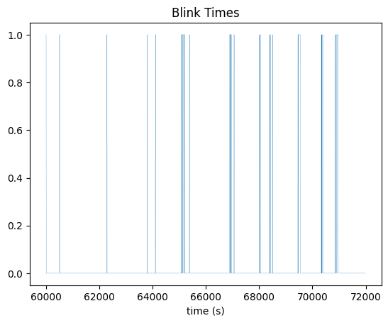
Blink Times#
fig, ax = plt.subplots()
ax.plot(time_axis, blink_times.data[start_idx:end_idx], linewidth=0.2)
ax.set_xlabel("time (s)")
ax.set_title("Blink Times")
Text(0.5, 1.0, 'Blink Times')
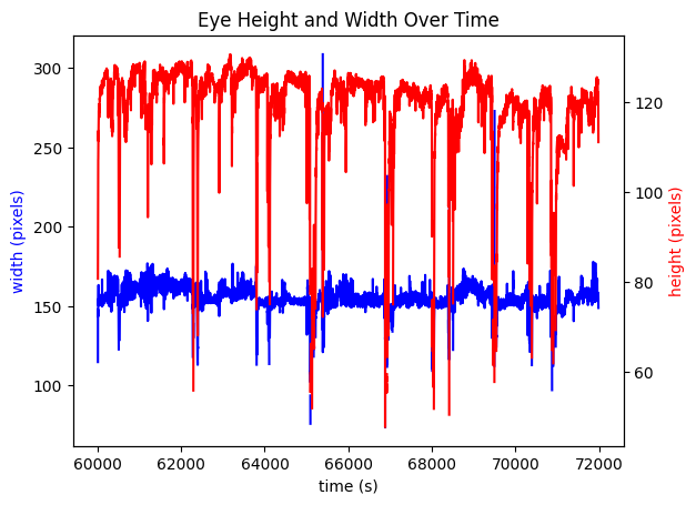
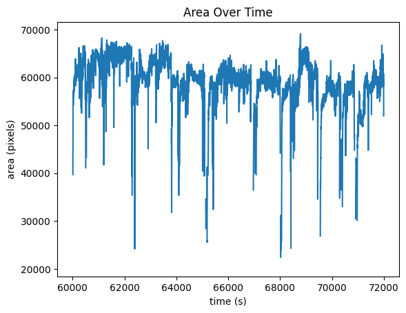
Area#
Below, eye height and width are plotted together, and area, the product of height and width, is also plotted. The units of height and width are defined in terms of pixels on the eye tracking camera.
fig, ax1 = plt.subplots()
ax1.set_xlabel('time (s)')
ax1.plot(time_axis, eye_tracking.width[start_idx:end_idx], color='b')
ax1.set_ylabel('width (pixels)', color='b')
ax2 = ax1.twinx()
ax2.plot(time_axis, eye_tracking.height[start_idx:end_idx], color='r')
ax2.set_ylabel('height (pixels)', color='r')
ax1.set_title("Eye Height and Width Over Time")
Text(0.5, 1.0, 'Eye Height and Width Over Time')
fig, ax1 = plt.subplots()
ax1.set_xlabel('time (s)')
ax1.set_ylabel('area (pixels)')
ax1.set_title("Area Over Time")
ax1.plot(time_axis, eye_tracking.area[start_idx:end_idx])
[<matplotlib.lines.Line2D at 0x1d2ced33b50>]
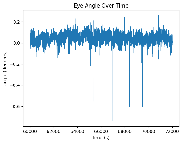
Angle#
fig, ax = plt.subplots()
angle = np.array(eye_tracking.angle)
ax.set_xlabel('time (s)')
ax.set_ylabel('angle (degrees)')
ax.set_title("Eye Angle Over Time")
ax.plot(time_axis, angle[start_idx:end_idx])
[<matplotlib.lines.Line2D at 0x1d2d2fe86d0>]
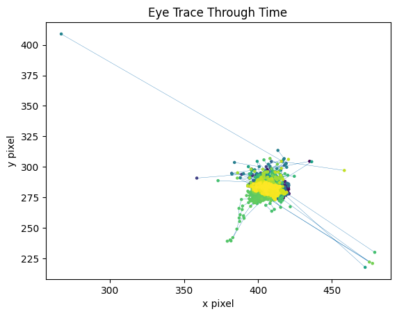
Eye Trace#
With marker color representing time, the x and y coordinates of the eye’s view are traced below.
# extract coords from eye tracking array
xs = np.array([point[0] for point in eye_tracking.data])
ys = np.array([point[1] for point in eye_tracking.data])
fig, ax = plt.subplots()
colors = plt.cm.viridis(np.linspace(0, 1, end_idx-start_idx))
ax.plot(xs[start_idx:end_idx], ys[start_idx:end_idx], zorder=0, linewidth=0.25)
ax.scatter(xs[start_idx:end_idx], ys[start_idx:end_idx], s=5, c=colors, zorder=1)

# change these to set the plot limits
# ax.set_xlim(310,360)
# ax.set_ylim(270,320)

ax.set_xlabel("x pixel")
ax.set_ylabel("y pixel")
ax.set_title("Eye Trace Through Time")
plt.show()
Running Data#
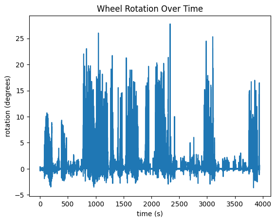
Apart from the Eye Tracking Data, the mouse’s running data is tracked in the "running" field of the processing section of the NWB File. Speed, in cm/s is tracked in the "speed" field. Another field, "dx" is also recorded which represents the number of degrees the wheel has turned between timestamp. These are plotted below. It is important to note that, at the moment, running data is stored in NWB differently in our Ecephys files and our Ophys files. Change the code in the cell below if you’re accessing a different type of file.
# swap these if you're accessing an Allen Ecephys file rather than a Ophys file
running_speed = nwb.processing["running"]["speed"]
# running_speed = nwb.processing["running"]["running_speed"]

wheel_rotation = nwb.processing["running"]["dx"]
# wheel_rotation = nwb.processing["running"]["running_wheel_rotation"]
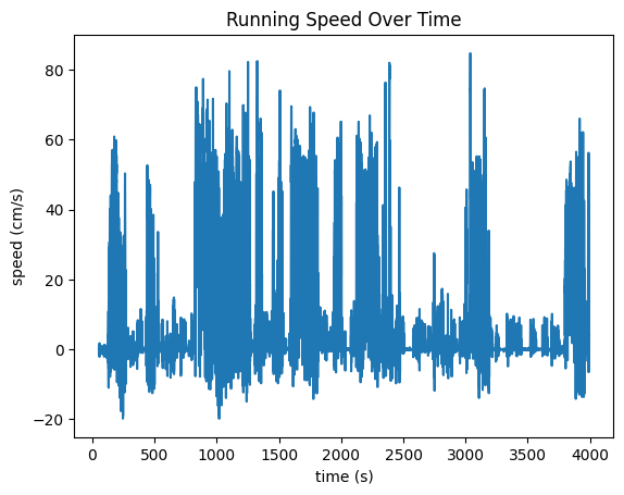
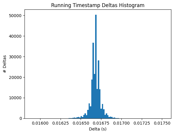
Running Speed#
Below are the running speed over time and wheel rotation over time. They should probably look very similar. Additionally, we show the distribution of the timestamp deltas. If the data was processed properly, there shouldn’t be many deviations. However, sometimes, individual frames might be dropped during processing from the experimental rigs which could show some diffs that are double what the expected value is.
speed_data = np.array(running_speed.data)
speed_timestamps = np.array(running_speed.timestamps)
print(speed_data.shape)
print(speed_timestamps.shape)

fig, ax = plt.subplots()
ax.set_xlabel("time (s)")
ax.set_ylabel("speed (cm/s)")
ax.set_title("Running Speed Over Time")
ax.plot(speed_timestamps, speed_data)
(236232,)
(236232,)
[<matplotlib.lines.Line2D at 0x1d2d31c2bc0>]
fig, ax = plt.subplots()
ax.hist(np.diff(speed_timestamps), 100)
ax.set_xlabel("Delta (s)")
ax.set_ylabel("# Deltas")
ax.set_title("Running Timestamp Deltas Histogram")
plt.show()
rotation_data = np.array(wheel_rotation.data[1:]) # cut out first value since it is high outlier
rotation_timestamps = np.array(wheel_rotation.timestamps[1:])
print(rotation_data.shape)
print(rotation_timestamps.shape)

fig, ax = plt.subplots()
ax.set_xlabel("time (s)")
ax.set_ylabel("rotation (degrees)")
ax.set_title("Wheel Rotation Over Time")
ax.plot(rotation_timestamps, rotation_data)
(236231,)
(236231,)
[<matplotlib.lines.Line2D at 0x1d2ccd6de70>]