Tensor Decomposition of Spiking Activity Through Trials

In several previous notebooks, we’ve utilized the Spike Matrix for analysis. As mentioned in Visualizing Unit Spikes, the Spike Matrix is a 3D matrix (or more precisely, a tensor) with dimensions neurons, time, and trials. Using the neuron spike trains and stimulus table from an NWB file, we can produce a spike matrix for a particular selection of neurons and stimulus trials. The paper [Williams et al., 2018] discusses TCA, a method for decomposing such a 3D spike matrix to yield components which isolate a set of features from the data. Each component consists of the three vectors called neuronal factors, temporal factors, and trial factors. In concert, these factors show a relationship between weighted populations of cells, their activity during the trials, and activity between trials. In contrast to PCA, TCA can be used to identify trends in neuron activity within trials as well as across trials. We do not aim to cover all uses of TCA, but rather help build a concrete intuition on how TCA can be used and pro and cons of this approach. The repo used for this is TensorTools

In this notebook, we demonstrate the simple usage of TCA and how it can be applied to our NWB files. First, cells are selected based on brain region and other criteria, then trials are selected based on repeats of specific trial movies. After this, the spike matrix is produced, and finally TCA produces decomposed factors and plots are generated to interpret them.

Environment Setup

try:
    from databook_utils.dandi_utils import dandi_download_open
except:
    !git clone https://github.com/AllenInstitute/openscope_databook.git
    %cd openscope_databook
    %pip install -e .

c:\Users\carter.peene\AppData\Local\Programs\Python\Python39\lib\site-packages\numpy\_distributor_init.py:30: UserWarning: loaded more than 1 DLL from .libs:
c:\Users\carter.peene\AppData\Local\Programs\Python\Python39\lib\site-packages\numpy\.libs\libopenblas.EL2C6PLE4ZYW3ECEVIV3OXXGRN2NRFM2.gfortran-win_amd64.dll
c:\Users\carter.peene\AppData\Local\Programs\Python\Python39\lib\site-packages\numpy\.libs\libopenblas.XWYDX2IKJW2NMTWSFYNGFUWKQU3LYTCZ.gfortran-win_amd64.dll
  warnings.warn("loaded more than 1 DLL from .libs:"

import os
import tensortools as tt
import numpy as np

import matplotlib.pyplot as plt

%matplotlib inline

Download File

For this notebook, the example file we use is from the Allen Institute’s Visual Coding - Neuropixels dataset. As long as the NWB file you choose has a properly formatted stimulus table and units table, this code should work.

dandiset_id = "000021"
dandi_filepath = "sub-717038285/sub-717038285_ses-732592105.nwb"
download_loc = "."
dandi_api_key = None

io = dandi_download_open(dandiset_id, dandi_filepath, download_loc, dandi_api_key=dandi_api_key)
nwb = io.read()

A newer version (0.56.2) of dandi/dandi-cli is available. You are using 0.55.1

File already exists
Opening file

c:\Users\carter.peene\AppData\Local\Programs\Python\Python39\lib\site-packages\hdmf\spec\namespace.py:531: UserWarning: Ignoring cached namespace 'hdmf-common' version 1.1.3 because version 1.8.0 is already loaded.
  warn("Ignoring cached namespace '%s' version %s because version %s is already loaded."
c:\Users\carter.peene\AppData\Local\Programs\Python\Python39\lib\site-packages\hdmf\spec\namespace.py:531: UserWarning: Ignoring cached namespace 'core' version 2.2.2 because version 2.5.0 is already loaded.
  warn("Ignoring cached namespace '%s' version %s because version %s is already loaded."

Selecting Units

To get more interesting factors, it may be of interest to just analyze a subset of Neurons of the NWB’s Units table. The helper function get_unit_locations is made from the Electrodes table to select units based on their brain region, and the possible brain regions to select from are printed. Here, units are selected from the regions VISp. VISl, and VISpm, and (for later purposes) the number of neurons in each region is recorded to n_neurons_in_region. To select units based on other criteria, you can write your own code in the cell below that begins with “selecting units spike times”.

units = nwb.units
units[:10]

	velocity_below	amplitude_cutoff	repolarization_slope	snr	firing_rate	waveform_duration	presence_ratio	isi_violations	cumulative_drift	spread	...	d_prime	cluster_id	amplitude	waveform_halfwidth	local_index	silhouette_score	nn_miss_rate	spike_times	spike_amplitudes	waveform_mean
id
915957951	-0.343384	0.000886	0.880810	4.800479	2.035908	0.686767	0.98	0.000000	53.49	50.0	...	6.214486	323	234.454545	0.137353	314	0.229600	0.000102	[58.4338983925338, 68.84436108646727, 69.12766...	[0.00035119779048895465, 0.0003151291869021440...	[[0.0, 0.2250300000000216, 2.9977350000000555,...
915957946	0.000000	0.000217	0.400703	3.429461	5.738931	0.714238	0.99	0.009670	123.55	50.0	...	6.316538	322	138.920730	0.151089	313	0.158374	0.000906	[1.021669806312146, 1.1772369117243047, 2.5084...	[0.00016757406732947436, 0.0001720397921770987...	[[0.0, -3.2106749999999806, 3.150420000000011,...
915957691	-1.103733	0.014154	0.426480	1.919786	2.008079	0.796650	0.99	2.705249	290.95	100.0	...	3.662792	275	147.761055	0.206030	268	0.158752	0.001013	[0.6530354333202749, 3.2586094484803794, 3.264...	[7.60907503923193e-05, 7.957109416173626e-05, ...	[[0.0, -11.971440000000083, -12.44139000000006...
915957685	-0.956569	0.000230	0.842665	4.186323	4.709665	0.837856	0.99	0.005385	53.80	90.0	...	5.161656	274	260.690625	0.192295	267	0.234811	0.000138	[1.2490037807948806, 1.2540371283237506, 1.831...	[0.000266164371359917, 0.0002605838430779542, ...	[[0.0, -5.997810000000001, 5.6064450000000186,...
915956513	0.343384	0.500000	0.562422	3.457604	2.181748	0.645561	0.99	0.209098	139.54	60.0	...	2.918675	43	221.177190	0.247236	43	0.057446	0.003356	[3.2777428357755536, 11.522366088064498, 12.26...	[0.000144906487588058, 0.00010868803407731714,...	[[0.0, 0.0228149999999836, 2.534804999999988, ...
915956508	1.030151	0.000004	0.958932	5.408729	6.252715	0.494472	0.99	0.001018	30.54	50.0	...	6.895246	42	322.610340	0.192295	42	0.212086	0.002584	[14.719841772563301, 22.41733014843588, 30.700...	[0.0002151604191262871, 0.00020362049040077184...	[[0.0, 7.416434999999929, 3.2403149999999847, ...
915956502	-1.030151	0.001222	0.513393	3.237491	16.870943	0.563149	0.99	0.031472	83.51	40.0	...	4.833891	41	187.746780	0.206030	41	0.218050	0.001938	[1.4603043767253872, 1.4698044035182873, 1.481...	[0.00015597232901272, 0.0002357881951492309, 0...	[[0.0, -1.0518299999999812, -1.572479999999974...
915957820	0.423506	0.500000	0.451907	3.245378	0.008816	0.192295	0.26	0.000000	0.00	90.0	...	2.035774	300	113.818916	0.109883	292	NaN	0.000000	[461.1188340837827, 4209.908773452706, 4513.18...	[6.916100951089473e-05, 0.00010573897883329469...	[[0.0, -7.005903614457829, -4.6729518072289125...
915957814	-0.686767	0.219911	0.377458	2.882758	2.044300	0.274707	0.91	0.152423	211.72	20.0	...	6.940011	299	90.401025	0.109883	291	0.063454	0.000170	[403.78390571557065, 540.1631903457029, 1001.0...	[8.160101108265708e-05, 8.231111987309405e-05,...	[[0.0, -2.198040000000006, 8.860604999999943, ...
915956679	0.240369	0.013547	0.198606	0.862630	0.497001	0.412060	0.99	56.734425	787.79	170.0	...	4.532952	73	61.062105	0.260972	73	NaN	0.000100	[32.79502608329068, 32.81382613631242, 32.8917...	[7.08162454791397e-05, 5.720387439876228e-05, ...	[[0.0, -0.5660849999999442, 1.869854999999987,...

10 rows × 29 columns

nwb.electrodes[:10]

	x	y	z	imp	location	filtering	group	group_name	probe_vertical_position	probe_horizontal_position	probe_id	local_index	valid_data
id
850229885	NaN	NaN	NaN	NaN	VISpm	AP band: 500 Hz high-pass; LFP band: 1000 Hz l...	probeB abc.EcephysElectrodeGroup at 0x30255172...	probeB	2380	43	733744647	236	True
850229827	NaN	NaN	NaN	NaN	grey	AP band: 500 Hz high-pass; LFP band: 1000 Hz l...	probeB abc.EcephysElectrodeGroup at 0x30255172...	probeB	2080	27	733744647	207	True
850230151	NaN	NaN	NaN	NaN		AP band: 500 Hz high-pass; LFP band: 1000 Hz l...	probeB abc.EcephysElectrodeGroup at 0x30255172...	probeB	3700	11	733744647	369	True
850229439	NaN	NaN	NaN	NaN	grey	AP band: 500 Hz high-pass; LFP band: 1000 Hz l...	probeB abc.EcephysElectrodeGroup at 0x30255172...	probeB	140	11	733744647	13	True
850229581	NaN	NaN	NaN	NaN	grey	AP band: 500 Hz high-pass; LFP band: 1000 Hz l...	probeB abc.EcephysElectrodeGroup at 0x30255172...	probeB	860	43	733744647	84	True
850229859	NaN	NaN	NaN	NaN	grey	AP band: 500 Hz high-pass; LFP band: 1000 Hz l...	probeB abc.EcephysElectrodeGroup at 0x30255172...	probeB	2240	27	733744647	223	True
850229457	NaN	NaN	NaN	NaN	grey	AP band: 500 Hz high-pass; LFP band: 1000 Hz l...	probeB abc.EcephysElectrodeGroup at 0x30255172...	probeB	240	59	733744647	22	True
850229815	NaN	NaN	NaN	NaN	grey	AP band: 500 Hz high-pass; LFP band: 1000 Hz l...	probeB abc.EcephysElectrodeGroup at 0x30255172...	probeB	2020	11	733744647	201	True
850230143	NaN	NaN	NaN	NaN		AP band: 500 Hz high-pass; LFP band: 1000 Hz l...	probeB abc.EcephysElectrodeGroup at 0x30255172...	probeB	3660	11	733744647	365	True
850229483	NaN	NaN	NaN	NaN	grey	AP band: 500 Hz high-pass; LFP band: 1000 Hz l...	probeB abc.EcephysElectrodeGroup at 0x30255172...	probeB	360	27	733744647	35	True

# select electrodes
channel_probes = {}

electrodes = nwb.electrodes
for i in range(len(electrodes)):
    channel_id = electrodes["id"][i]
    location = electrodes["location"][i]
    channel_probes[channel_id] = location

# function aligns location information from electrodes table with channel id from the units table
def get_unit_location(row):
    return channel_probes[int(row.peak_channel_id)]

print(set(get_unit_location(row) for row in units))

{'', 'VISl', 'VISal', 'VISpm', 'VISrl', 'VISp', 'grey'}

### selecting units spike times

units_spike_times = units["spike_times"]
brain_regions = ["VISp", "VISl", "VISpm"]

# select units based if they have 'good' quality and exists in one of the specified brain_regions
units_spike_times = []
n_neurons_in_region = []
# for the output plots below it is important here that the `units_spike_times` array is partitioned based on each neuron's brain region
for location in brain_regions:
    location_units_spike_times = []
    for row in units:
        if get_unit_location(row) == location and row.quality.item() == "good":
            location_units_spike_times.append(row.spike_times.item())
    
    # used for distinguishing brain regions in the output plots
    n_neurons_in_region.append(len(location_units_spike_times))
    # sort neurons by depth within brain region


    units_spike_times += location_units_spike_times

print(len(units_spike_times))
print(n_neurons_in_region)

604
[244, 206, 154]

Selecting Stimulus Trials

Here the stimulus times of the trials of interest are selected from one of the NWB’s Intervals tables. Below are printed the keys for each Intervals table. In this example natural_movie_one_presentations is selected for its high repetition and the fact that natural stimuli often evoke very reliable responses. You can modify the stim_select cell below to change the criteria for select stimulus times. The output should be a stim_times list of timestamps that the stimulus was presented. In this example it can be seen that there is a large gap between the 9th and 10th stim times.

nwb.intervals.keys()

dict_keys(['drifting_gratings_presentations', 'flashes_presentations', 'gabors_presentations', 'invalid_times', 'natural_movie_one_presentations', 'natural_movie_three_presentations', 'natural_scenes_presentations', 'spontaneous_presentations', 'static_gratings_presentations'])

# stim_table = nwb.intervals["static_gratings_presentations"]
stim_table = nwb.intervals["natural_movie_one_presentations"]
stim_table[0:10]

	start_time	stop_time	stimulus_name	stimulus_block	color	opacity	size	units	stimulus_index	orientation	frame	contrast	tags	timeseries
id
0	2843.937384	2843.970745	natural_movie_one	4.0	[1.0, 1.0, 1.0]	1.0	[1920.0, 1080.0]	pix	3.0	0.0	0.0	1.0	[stimulus_time_interval]	[(22000, 1, timestamps pynwb.base.TimeSeries a...
1	2843.970745	2844.004106	natural_movie_one	4.0	[1.0, 1.0, 1.0]	1.0	[1920.0, 1080.0]	pix	3.0	0.0	1.0	1.0	[stimulus_time_interval]	[(22001, 1, timestamps pynwb.base.TimeSeries a...
2	2844.004106	2844.037466	natural_movie_one	4.0	[1.0, 1.0, 1.0]	1.0	[1920.0, 1080.0]	pix	3.0	0.0	2.0	1.0	[stimulus_time_interval]	[(22002, 1, timestamps pynwb.base.TimeSeries a...
3	2844.037466	2844.070827	natural_movie_one	4.0	[1.0, 1.0, 1.0]	1.0	[1920.0, 1080.0]	pix	3.0	0.0	3.0	1.0	[stimulus_time_interval]	[(22003, 1, timestamps pynwb.base.TimeSeries a...
4	2844.070827	2844.104188	natural_movie_one	4.0	[1.0, 1.0, 1.0]	1.0	[1920.0, 1080.0]	pix	3.0	0.0	4.0	1.0	[stimulus_time_interval]	[(22004, 1, timestamps pynwb.base.TimeSeries a...
5	2844.104188	2844.137549	natural_movie_one	4.0	[1.0, 1.0, 1.0]	1.0	[1920.0, 1080.0]	pix	3.0	0.0	5.0	1.0	[stimulus_time_interval]	[(22005, 1, timestamps pynwb.base.TimeSeries a...
6	2844.137549	2844.170909	natural_movie_one	4.0	[1.0, 1.0, 1.0]	1.0	[1920.0, 1080.0]	pix	3.0	0.0	6.0	1.0	[stimulus_time_interval]	[(22006, 1, timestamps pynwb.base.TimeSeries a...
7	2844.170909	2844.204270	natural_movie_one	4.0	[1.0, 1.0, 1.0]	1.0	[1920.0, 1080.0]	pix	3.0	0.0	7.0	1.0	[stimulus_time_interval]	[(22007, 1, timestamps pynwb.base.TimeSeries a...
8	2844.204270	2844.237631	natural_movie_one	4.0	[1.0, 1.0, 1.0]	1.0	[1920.0, 1080.0]	pix	3.0	0.0	8.0	1.0	[stimulus_time_interval]	[(22008, 1, timestamps pynwb.base.TimeSeries a...
9	2844.237631	2844.270991	natural_movie_one	4.0	[1.0, 1.0, 1.0]	1.0	[1920.0, 1080.0]	pix	3.0	0.0	9.0	1.0	[stimulus_time_interval]	[(22009, 1, timestamps pynwb.base.TimeSeries a...

### select stimulus based on

stim_select = lambda row: int(row.frame) == 0
stim_times = [float(stim_table[i].start_time) for i in range(len(stim_table)) if stim_select(stim_table[i])]

# stim_times = []
# for i in range(len(stim_table)):
#     if i == len(stim_table)-2:
#         break
#     if float(stim_table[i].color) == -1 and float(stim_table[i+1].color) == 1:
#         stim_times.append(stim_table[i].stop_time.item())

print(len(stim_times))

20

Spike Matrix

Here the Spike Matrix is produced using the selected neuron spike trains and stimulus times. Some important parameters must be set to devise this matrix. Set time_resolution to be the bin size (in seconds) that’s used to count the spikes. Set window_start_time and window_end_time to be the bounds (in seconds, relative to the stimulus event) of the stimulus period to analyze. This outputs the three dimensional spike matrix ready for analyze.

# # bin size for counting spikes
time_resolution = 0.2

# # start and end times (relative to the stimulus at 0 seconds) that we want to examine and align spikes to
window_start_time = 0
window_end_time = 5

def get_spike_matrix(units_spike_times, stim_times, bin_edges, time_resolution):
    n_units = len(units_spike_times)
    n_trials = len(stim_times)

    # 3D spike matrix to be populated with spike counts
    spike_matrix = np.zeros((n_units, len(bin_edges), n_trials))

    # populate 3D spike matrix for each unit for each stimulus trial by counting spikes into bins
    for unit_idx in range(n_units):
        spike_times = units_spike_times[unit_idx]

        for stim_idx, stim_time in enumerate(stim_times):
            # get spike times that fall within the bin's time range relative to the stim time        
            first_bin_time = stim_time + bin_edges[0]
            last_bin_time = stim_time + bin_edges[-1]
            first_spike_in_range, last_spike_in_range = np.searchsorted(spike_times, [first_bin_time, last_bin_time])
            spike_times_in_range = spike_times[first_spike_in_range:last_spike_in_range]

            # convert spike times into relative time bin indices
            bin_indices = ((spike_times_in_range - (first_bin_time)) / time_resolution).astype(int)
            
            # mark that there is a spike at these bin times for this unit on this stim trial
            for bin_idx in bin_indices:
                spike_matrix[unit_idx, bin_idx, stim_idx] += 1

    return spike_matrix

# time bins used
n_bins = int((window_end_time - window_start_time) / time_resolution)
bin_edges = np.linspace(window_start_time, window_end_time, n_bins, endpoint=True)

stim_times = stim_times[:20]
spike_matrix = get_spike_matrix(units_spike_times, stim_times, bin_edges, time_resolution)
spike_matrix.shape

(604, 25, 20)

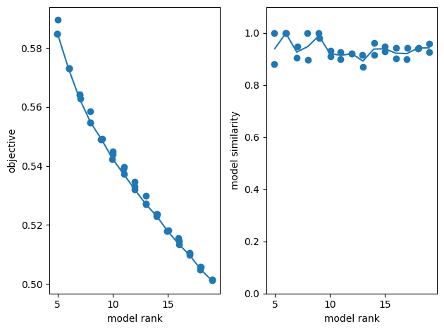
Running TCA

After the spike matrix is produced, it is a simple matter to run the decomposition step. The model is instantiated with the tt.Ensemble method. Since the number of components can have a significant output on the quality of your decomposition, a range of ranks can be specified in order to produce many decompositions, and replicates can be set to run multiple replicates of each rank. TensorTools can produce objective and similarity plots which after fitting which display the relationship between the number of ranks, performance, and number of replicates to better tune these parameters for your analysis. Below, the model is fit with 5 to 15 ranks and their objective and similarity plots are shown.

TCA will identify correlations across neurons trials and time to build a number of components that maximize the ability to reconstruct the original data matrix. It is therefore essential to use scientific judgement when using this tool. There are two main decisions to make: The final rank to use and making sure that the extracted model is faithfully representing the neuronal activity.

Choosing a final rank is a complex question with no “one-size fits all” answer. Generally, as the rank increases, the objective will decrease as more degrees of freedom allows for better reconstructions. Higher rank models also are more computational expensive to compute.

In some cases, if the rank is too low, you could end up with unreliable models. The model similarity plot is useful to make this evaluation as each dot represents a given model run. A good practice is to pick a rank high enough that provides reliable, similar models at each run. Beyond that, you should use your scientific judgement and choose a rank that allow you to conduct your analysis in practice. If your goal is to identify broader components shared across many neurons, a lower rank might be more appropriate. Increasing the rank will further sub-divide components, improving the objective, but will not provide additional insights. Eventually you can test the sensibility of your analysis against this choice with cross-validation.

ensemble = tt.Ensemble(fit_method="ncp_hals")
ensemble.fit(spike_matrix, ranks=range(5,20), replicates=3)

fig, axes = plt.subplots(1, 2)
tt.plot_objective(ensemble, ax=axes[0])   # plot reconstruction error as a function of num components.
tt.plot_similarity(ensemble, ax=axes[1])  # plot model similarity as a function of num components.
fig.tight_layout()

plt.show()

Fitting rank-5 models:   0%|          | 0/3 [00:00<?, ?it/s]c:\Users\carter.peene\AppData\Local\Programs\Python\Python39\lib\site-packages\tensortools\optimize\ncp_hals.py:185: NumbaPerformanceWarning: '@' is faster on contiguous arrays, called on (Array(float64, 2, 'C', False, aligned=True), Array(float64, 1, 'A', False, aligned=True))
  Cp = factors[:, idx] @ grams[idx][:, p]
                                                                    

Rank-5 models:  min obj, 0.59;  max obj, 0.59;  time to fit, 5.8s

Rank-6 models:  min obj, 0.58;  max obj, 0.58;  time to fit, 0.3s

Rank-7 models:  min obj, 0.57;  max obj, 0.57;  time to fit, 0.3s

Rank-8 models:  min obj, 0.56;  max obj, 0.56;  time to fit, 0.7s

Rank-9 models:  min obj, 0.55;  max obj, 0.55;  time to fit, 0.9s

Rank-10 models:  min obj, 0.55;  max obj, 0.55;  time to fit, 1.0s

Rank-11 models:  min obj, 0.54;  max obj, 0.54;  time to fit, 1.1s

Rank-12 models:  min obj, 0.54;  max obj, 0.54;  time to fit, 0.9s

Rank-13 models:  min obj, 0.53;  max obj, 0.53;  time to fit, 1.1s

Rank-14 models:  min obj, 0.53;  max obj, 0.53;  time to fit, 0.9s

Rank-15 models:  min obj, 0.52;  max obj, 0.52;  time to fit, 1.2s

Rank-16 models:  min obj, 0.52;  max obj, 0.52;  time to fit, 1.2s

Rank-17 models:  min obj, 0.51;  max obj, 0.51;  time to fit, 4.0s

Rank-18 models:  min obj, 0.51;  max obj, 0.51;  time to fit, 3.4s

Rank-19 models:  min obj, 0.50;  max obj, 0.51;  time to fit, 3.5s

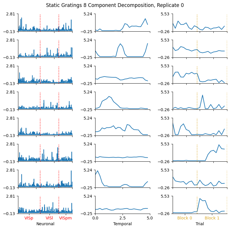
Showing the Components

The factors for a given rank and replicate are retrieved from the ensemble’s factors method. Set num_components and replicate to be the indices you’re interested from the model’s various fits. TensorTools also has a native function for plotting the selected model called plot_factors. However, this is not as decorated as we would prefer for our purposes, so here is defined plot_factors_fancy which takes the figure and subplots from TensorTools and adds some extra labeling. Specifically, it display the partitioning of the neuronal factors based on their brain region, and partitioning the two main stimulus epochs from this particular experiment. It can be seen in the components plot below that, for some factors, there is differential activity of the neurons between each brain region. The same can be said for the trial factors between the first block of stimulus trials and the second block.

This given run already provide interesting insights with regards to the neuronal activity during repeats of the natural movies. Our movie was shown in 2 blocks : Block 0 and 1, each made of successive repeats of the movie. These blocks are identified on the previous plot with a yellow dashed line. TCA identifies several components that are block specific and sometime transiently activated at the onset of the first or second block. Certain components are evenly distributed across all trials, are non-homogenously distributed across cells (in VISp, VISl, VISpm) and show very strong transient patterns of activity. Those components could be related to specific aspects of the movie.

# Plot the low-d factors for an example model, e.g. rank-2, first optimization run / replicate.
num_components = 8
replicate = 0

def plot_factors_fancy(fig, subplots, n_neurons_in_region, stim_times, window_start_time, window_end_time, title=None, stim_borders_thresh=-1):
  # get lines separating the neurons of the selected brain regions and their midpoints for label locations
  region_bounds = np.array( [0] + [sum(n_neurons_in_region[:i+1]) for i in range(len(n_neurons_in_region))] )
  region_lines = region_bounds[1:-1]
  region_label_locs = region_bounds[:-1] + np.diff(region_bounds)/2

  # get lines separating blocks of stimulus repeats and their midpoints for label locations
  if stim_borders_thresh > 0:
    stim_diffs = np.diff(stim_times)
    stim_gaps, = np.where(stim_diffs > stim_borders_thresh*np.median(stim_diffs))
    stim_bounds = [0] + list(stim_gaps) + [len(stim_times)]
    stim_label_locs = stim_bounds[:-1] + np.diff(stim_bounds)/2
    stim_block_labels = [f"Block {i}" for i in range(len(stim_label_locs))]

  for subplot in subplots:
    # draw lines separating brain regions
    n_ymin, n_ymax = subplot[0].get_ylim()
    subplot[0].vlines(region_lines, n_ymin, n_ymax, ls=":", color="red")

    t_xmin, t_xmax = subplot[1].get_xlim()
    subplot[1].set_xticks(np.linspace(t_xmin, t_xmax, 3), labels=np.linspace(window_start_time, window_end_time, 3))

    # draw lines separating trial intervals
    if stim_borders_thresh > 0:
        ymin, ymax = subplot[2].get_ylim()
        subplot[2].vlines(stim_bounds, ymin, ymax, ls=":", color="goldenrod")

  # set tick labels for brain regions
  subplot[0].set_xticks(region_label_locs, brain_regions)
  [t.set_color("red") for t in subplot[0].xaxis.get_ticklabels()]

  # set tick labels for blocks of stimulus repeats
  if stim_borders_thresh > 0:
    subplots[-1][2].set_xticks(stim_label_locs, stim_block_labels)
    [t.set_color("goldenrod") for t in subplot[2].xaxis.get_ticklabels()]

  subplots[-1][0].set_xlabel("Neuronal")
  subplots[-1][1].set_xlabel("Temporal")
  subplots[-1][2].set_xlabel("Trial")

  fig.suptitle(title)
  fig.tight_layout()
  plt.show()

factor = ensemble.factors(num_components)[replicate]
fig, subplots, lines = tt.plot_factors(factor)  # plot the low-d factors
title = f"Static Gratings {num_components} Component Decomposition, Replicate {replicate}"

plot_factors_fancy(fig, subplots, n_neurons_in_region, stim_times, window_start_time, window_end_time, title=title, stim_borders_thresh=10)

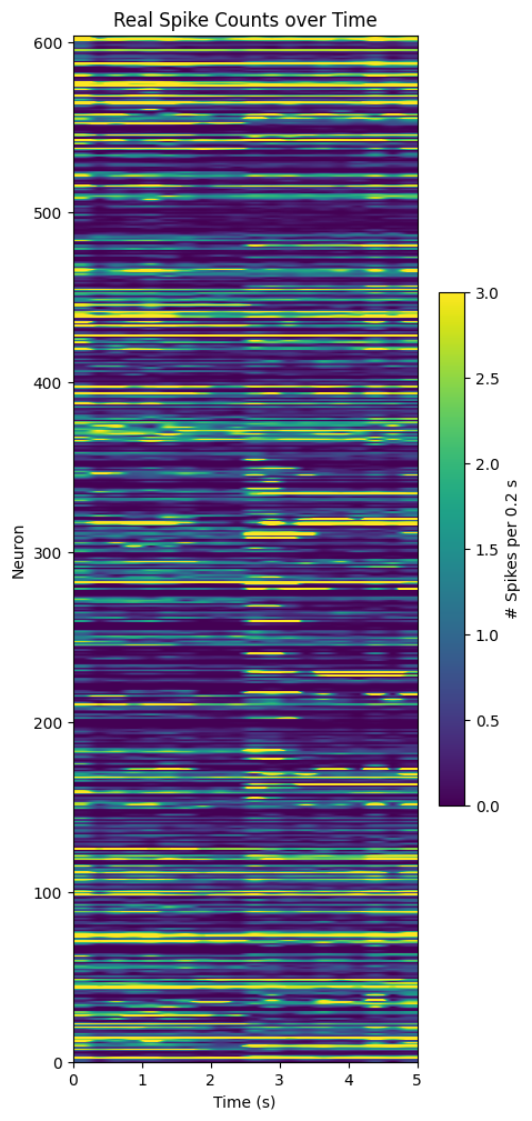
Extracting Activity

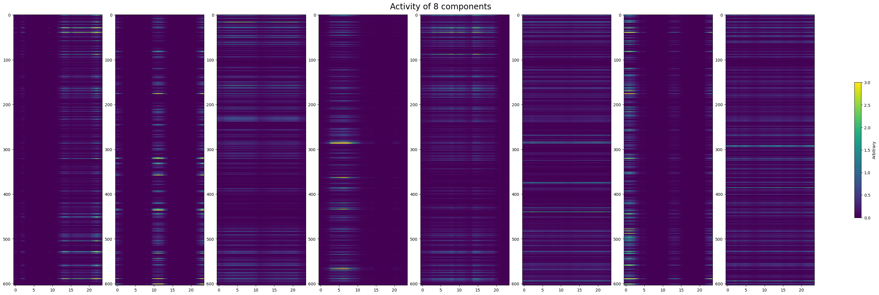
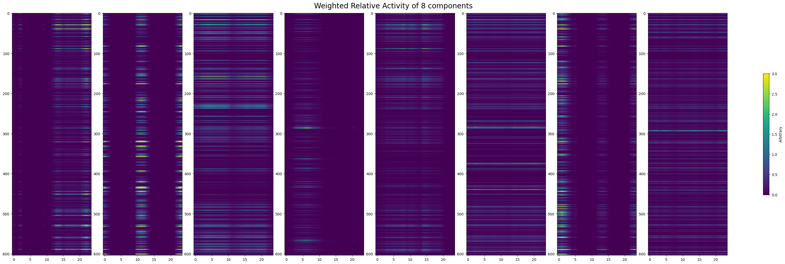
Next, we try to verify if the component representations are really reflected in the data. You can select specific components by setting selected_components to a list of component indices from the plot above. Below the real spiking activity over for all cells is shown from the spike matrix that was inputted to TCA. Below that, the selected temporal components are plotted in 2D with their respective neuronal weights to resemble the real spike counts plot. Visually, we can disentangle the various components’ effect on the overall spike counts. Because different components also vary in their impact throughout trials, we also show each of the components weighted by their overall contribution to the spike counts.

# components of interest from the plot above
selected_components = [0,1,2,3,4,5,6,7]

def get_component_spike_counts(factor, component, units_spike_times):
    neuron_component = factor[0][:, component]

    # get indices of greatest 10% neurons
    frac = len(neuron_component) // 10
    max_idxs = np.argpartition(neuron_component, -frac)[-frac:]

    # subselect these units from units_spike_times
    selected_units_spike_times = units_spike_times[max_idxs]
    len(selected_units_spike_times)

    selected_spikes = get_spike_matrix(selected_units_spike_times, stim_times, bin_edges, time_resolution)
    spike_counts = np.mean(selected_spikes, axis=2)
    return spike_counts

spike_counts = np.mean(spike_matrix, axis=2)
fig, ax = plt.subplots(figsize=(5,12))
im = ax.imshow(spike_counts, extent=[window_start_time,window_end_time,0,len(spike_counts)], aspect="auto", vmin=0, vmax=3)

cbar = fig.colorbar(im, shrink=0.5)
cbar.set_label(f"# Spikes per {time_resolution} s")

ax.set_title("Real Spike Counts over Time")
ax.set_xlabel("Time (s)")
ax.set_ylabel("Neuron")

Text(0, 0.5, 'Neuron')

fig, axes = plt.subplots(1, len(selected_components), figsize=(30,10), constrained_layout=True)
for i in range(len(selected_components)):
    component_idx = selected_components[i]
    neuron_component = factor[0][:, component_idx]
    time_component = factor[1][:, component_idx]

    transformed_neuron_component = np.expand_dims(neuron_component, 1)
    neuron_weighted_time_component = time_component * transformed_neuron_component
    im = axes[i].imshow(neuron_weighted_time_component, aspect="auto", vmin=0, vmax=3)

cbar = fig.colorbar(im, ax=axes.flatten(), shrink=0.5)
cbar.set_label("Arbitrary")
fig.suptitle(f"Activity of {len(axes)} components", size=20)

Text(0.5, 0.98, 'Activity of 8 components')

fig, axes = plt.subplots(1, len(selected_components), figsize=(30,10), constrained_layout=True)
for i in range(len(selected_components)):
    component_idx = selected_components[i]
    neuron_component = factor[0][:, component_idx]
    time_component = factor[1][:, component_idx]
    trial_component = factor[2][:, component_idx]

    transformed_neuron_component = np.expand_dims(neuron_component, 1)
    neuron_weighted_time_component = time_component * transformed_neuron_component
    
    trial_component_weight = np.mean(trial_component)
    trial_weighted_times = neuron_weighted_time_component * trial_component_weight
    im = axes[i].imshow(trial_weighted_times, aspect="auto", vmin=0, vmax=3)

cbar = fig.colorbar(im, ax=axes.flatten(), shrink=0.5)
cbar.set_label("Arbitrary")
fig.suptitle(f"Weighted Relative Activity of {len(axes)} components", size=20)

Text(0.5, 0.98, 'Weighted Relative Activity of 8 components')

Comparing Different Stimuli

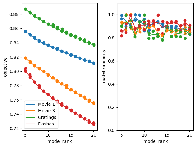
TCA’s performance varies. Here, we produce a spike matrix and run TCA on four different stimulus types included in this file. For comparison’s sake, they all use a 0.25 second period following the selected stimulus times with a bin size of 10 ms. The stimuli used are natural movies 1, natural movies 3, gratings, and full field flashes. In the loss plot following the training, we can compare TCA’s relative performance between all these stim types. This example would seem to suggest that flashes is inherently processed in a ‘lower dimensional’ space than the rest, followed by movie 3, movie 1 and finally gratings, which is thus the most complex. It could also be the case that different bin sizes and stim window length would be better at capturing the responses to a particular stimulus. This will depend on the speed and number of trials of the stimulus regimen used, which can be gleaned from each stimulus’ respective stim table.

time_resolution = 0.01
window_start_time = 0
window_end_time = 0.25

def train_ensemble(units_spike_times, stim_times, bin_edges, time_resolution):
    spike_matrix = get_spike_matrix(units_spike_times, stim_times, bin_edges, time_resolution)
    print(spike_matrix.shape)

    ensemble = tt.Ensemble(fit_method="ncp_hals")
    ensemble.fit(spike_matrix, ranks=range(5,21), replicates=3)
    return ensemble

def compare_ensembles(ensembles, names, obj_ax, sim_ax):
    for ensemble in ensembles:
        tt.plot_objective(ensemble, ax=obj_ax)   # plot reconstruction error as a function of num components.
        tt.plot_similarity(ensemble, ax=sim_ax)  # plot model similarity as a function of num components.

    lines = obj_ax.lines
    obj_ax.legend(lines, names)

def train_four_ensembles(nwb, time_resolution, window_start_time, window_end_time):
    # make sure ensembles share the same temporal axis for proper comparison
    n_bins = int((window_end_time - window_start_time) / time_resolution)
    bin_edges = np.linspace(window_start_time, window_end_time, n_bins, endpoint=True)

    stim_table_1 = nwb.intervals["natural_movie_one_presentations"]
    stim_select_1 = lambda row: int(row.frame) == 0
    stim_times_1 = [float(stim_table_1[i].start_time) for i in range(len(stim_table_1)) if stim_select_1(stim_table_1[i])]

    stim_table_2 = nwb.intervals["natural_movie_three_presentations"]
    stim_select_2 = lambda row: int(row.frame) == 0
    stim_times_2 = [float(stim_table_2[i].start_time) for i in range(len(stim_table_2)) if stim_select_2(stim_table_2[i])]

    stim_table_3 = nwb.intervals["static_gratings_presentations"]
    stim_select_3 = lambda row: float(row.orientation) == 90.0 and float(row.phase) == 0.5
    stim_times_3 = [float(stim_table_3[i].start_time) for i in range(len(stim_table_3)) if stim_select_3(stim_table_3[i])]

    stim_table_4 = nwb.intervals["flashes_presentations"]
    stim_times_4 = []
    for i in range(len(stim_table_4)):
        if i == len(stim_table_4)-2:
            break
        if float(stim_table_4[i].color) == -1 and float(stim_table_4[i+1].color) == 1:
            stim_times_4.append(stim_table_4[i].stop_time.item())

    # shorten number of stim times to fewest so all models have the same number of trials for a proper comparison
    # min_trials = min(len(stim_times_1), len(stim_times_2), len(stim_times_3), len(stim_times_4))
    min_trials = 20
    stim_times_1 = stim_times_1[:min_trials]
    stim_times_2 = stim_times_2[:min_trials]
    stim_times_3 = stim_times_3[:min_trials]
    stim_times_4 = stim_times_4[:min_trials]

    # train the ensembles for each stim type on the selected stim times
    ensemble_1 = train_ensemble(units_spike_times, stim_times_1, bin_edges, time_resolution)
    ensemble_2 = train_ensemble(units_spike_times, stim_times_2, bin_edges, time_resolution)
    ensemble_3 = train_ensemble(units_spike_times, stim_times_3, bin_edges, time_resolution)
    ensemble_4 = train_ensemble(units_spike_times, stim_times_4, bin_edges, time_resolution)

    return ensemble_1, ensemble_2, ensemble_3, ensemble_4

%%capture
ensembles = train_four_ensembles(nwb, time_resolution, window_start_time, window_end_time)
fig, axes = plt.subplots(1,2)
compare_ensembles(ensembles, ["Movie 1","Movie 3","Gratings","Flashes"], axes[0], axes[1]);

fig.tight_layout()
fig

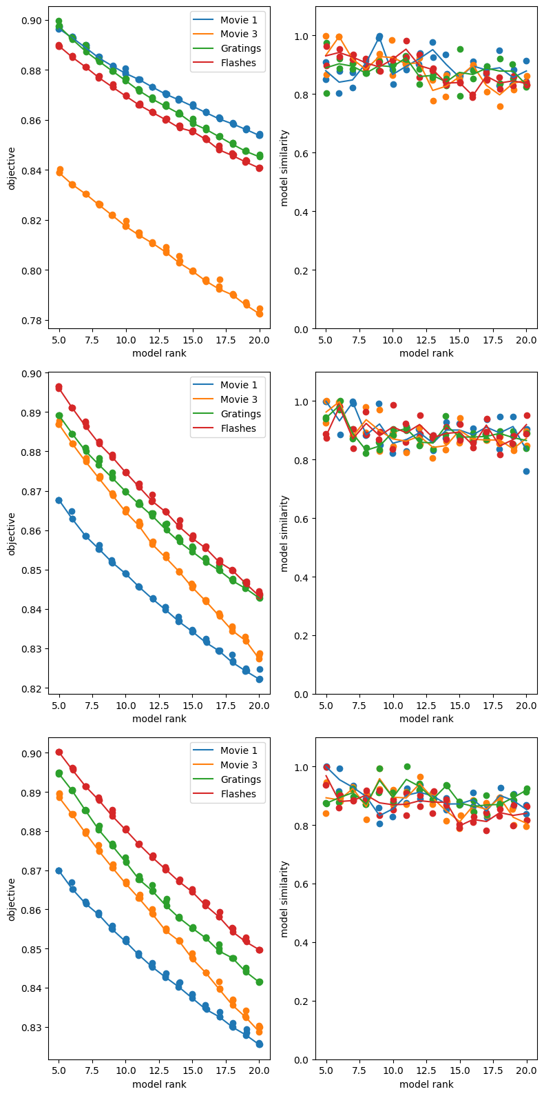
Comparing With Other Sessions

We can run this analysis on other files and view how the dimensionality of the different stimuli compares for other mice in other sessions. For this data, it can be seen that there is not a strongly consistent order between sessions of the different stimuli. Playing around with a few parameters can change this pattern; lengthening the the window and bin size with window_start_time, window_end_time, and time_resolution will affect how well TCA fits different stims. This is expected because different time window lengths will capture different response dynamics. For instance, a time window that is 2 seconds won’t do a very good job at capturing responses to flashes or gratings, which occur on the ms timescale. Typically, having more time bins will make the model fit worse, but may improve the quality of the insights yielded. This is because fewer time bins will be simpler and easier to reduce dimensionality.

Additionally, it can be seen below that the number of components can have a big impact on the resulting representations. While all stimuli are fit better with more components, some have a stronger fit than others with the same number of components.

%%capture
filepaths = ["sub-718643564/sub-718643564_ses-737581020.nwb", "sub-719817799/sub-719817799_ses-744228101.nwb", "sub-722882751/sub-722882751_ses-743475441.nwb"]

fig, axes = plt.subplots(len(filepaths),2, figsize=(8,16))
for i, filepath in enumerate(filepaths):
    io = dandi_download_open(dandiset_id, filepath, download_loc, dandi_api_key=dandi_api_key)
    nwb = io.read()
    ensembles = train_four_ensembles(nwb, time_resolution, window_start_time, window_end_time)
    compare_ensembles(ensembles, ["Movie 1","Movie 3","Gratings","Flashes"], axes[i][0], axes[i][1])

fig.tight_layout()
fig