OpenScope’s Global/Local Oddball Dataset

Current state of knowledge in the field: The brain rapidly adapts to unchanging environments, and is most excited by surprising events. A leading model to explain this phenomenon is predictive coding. Predictive coding proposes that the brain compares incoming sensory information against a prediction signal. This prediction is based on an internal model that is generated in higher-order cortex. This model reflects the brain’s assumptions about the statistics of the environment. If an incoming sensory signal matches the prediction, the two signals cancel. Expected sensory data thus are “explained away” and leave the brain unexcited. In other words, predictive coding is subtractive. The prediction signal inhibits the processing of sensory data.

Whenever the sensory signal does not match the prediction, subtraction results in a larger value, called the prediction error. This error signal initiates excitation in lower-order cortex that propagates feedforward up the cortical hierarchy (i.e., V1, RL, LM, AL, PM, and AM). Prediction errors then instigate updates to the internal model to improve future predictions. Associated prediction update signals flow back down the hierarchy. Consistent with this model, optogenetic silencing of top-down inputs from frontal to visual cortex largely eliminates prediction error signals. However, the precise circuit mechanisms that generate these signals are largely unknown. The GLO projects aims close this knowledge gap. Specifically, by recording from multiple neuropixels across the visual cortical hierarchy, we will uncover what information is carried by layer 2 and 3 spikes that feed forward vs. by layer 5 and 6 spikes that feed back, using recently established analytic tools. To fully understand the involved neural mechanisms, we propose to go further: It is now possible to measure specific populations of inhibitory interneurons in tasks manipulating stimulus predictability using two-photon Calcium imaging. This technique revealed distinct computations for somatostatin (SOM+) vs. parvalbumin (PV+) interneurons in mice exposed to the same repeated (and thus predictable) stimulus. As stimuli became increasingly predictable, PV+ interneurons became less active while SOM+ interneurons became more active. Thus, the subtraction between predicted stimuli and sensory data seems to be mediated by SOM+ interneurons. This observation also implies that PV+ interneurons might be involved in the generation of prediction errors. However, this work relied on stimulus repetitions across several days, thus lacking insight into the dynamics on a more behaviorally relevant scale.

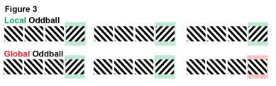
Lastly, the project aims to answer one of the most vexing paradigmatic questions of predictive coding: Significant progress in our understanding of the neural machinery underlying predictive coding stems from so-called oddball tasks. Specifically, by differentiating between so-called local (1st order) vs. global (2nd order) oddballs, researchers successfully dissociated automatic mechanisms of prediction from context-driven forms of predictive processing (Fig. 3). Cortical responses to local oddballs occur reflexively, even under deep anesthesia. Cortical responses to global oddballs require integration of stimuli across time to form complex predictions and are absent during unconsciousness. However, little is known about the neural circuitry supporting these two types of prediction errors. As we lay out below, the multi-area laminar spiking data combined with optogenetic cell type characterization (optotagging) of the Allen Institute can close this gap. Using this combination, we will specify the laminar sources, inhibitory cell types, and directions of neural signal flow (feedforward/feedback) that mediate these computations.

Environment Setup

⚠️Note: If running on a new environment, run this cell once and then restart the kernel⚠️

import warnings
warnings.filterwarnings('ignore')

try:
    from databook_utils.dandi_utils import dandi_download_open
except:
    !git clone https://github.com/AllenInstitute/openscope_databook.git
    %cd openscope_databook
    %pip install -e .
    %cd docs/projects

import os

import matplotlib as mpl
import matplotlib.pyplot as plt
import numpy as np
import pandas as pd

from math import floor, ceil, isclose
from PIL import Image

The Experiment

As shown in the metadata table below, Openscope’s GLO Experiment has produced 15 main files on the DANDI Archive, with 5 males and 10 females. There are no wildtype mice but there are Pvalb and Sst genotypes. This table was generated from Getting Experimental Metadata from DANDI.

session_files = pd.read_csv("../../data/glo_sessions.csv")
session_files

	identifier	size	path	session_time	specimen_name	sex	age	genotype	probes	stim_types	n_units	session_end
0	89fa5067-31a8-4f2d-a043-5721120501a0	2499178105	sub-621890/sub-621890_ses-1186358749_ogen.nwb	2022-06-22 00:00:00-07:00	621890	F	128	Sst-IRES-Cre/wt;Ai32(RCL-ChR2(H134R)_EYFP)/wt	{'probeF', 'probeA', 'probeB', 'probeD', 'prob...	{'init_grating_presentations', 'create_recepti...	2446	6713.70871
1	463e9cae-ff12-4e54-8b8f-e9293480f762	982474234	sub-621891/sub-621891_ses-1179909741_ogen.nwb	2022-05-25 00:00:00-07:00	621891	F	100	Sst-IRES-Cre/wt;Ai32(RCL-ChR2(H134R)_EYFP)/wt	{'probeD', 'OptogeneticStimulusDevice', 'probe...	{'init_grating_presentations', 'create_recepti...	1118	6713.54730
2	38e79b1b-e2a6-4f5c-ae62-5538d295b827	2341394409	sub-632487/sub-632487_ses-1204677304_ogen.nwb	2022-09-01 00:00:00-07:00	632487	F	122	Sst-IRES-Cre/wt;Ai32(RCL-ChR2(H134R)_EYFP)/wt	{'probeF', 'probeA', 'probeB', 'probeD', 'prob...	{'init_grating_presentations', 'create_recepti...	2745	6948.51640
3	2b44dc78-2c9f-4a71-95ed-360df2b70d61	2180444622	sub-637542/sub-637542_ses-1211241460_ogen.nwb	2022-09-15 00:00:00-07:00	637542	F	98	Pvalb-IRES-Cre/wt;Ai32(RCL-ChR2(H134R)_EYFP)/wt	{'probeF', 'probeA', 'probeB', 'probeD', 'prob...	{'init_grating_presentations', 'create_recepti...	2055	7012.67225
4	b305ccec-fa84-445e-aea5-0126d6eff558	2456101222	sub-632485/sub-632485_ses-1203581890_ogen.nwb	2022-08-31 00:00:00-07:00	632485	F	121	Sst-IRES-Cre/wt;Ai32(RCL-ChR2(H134R)_EYFP)/wt	{'probeF', 'probeA', 'probeB', 'probeD', 'prob...	{'init_grating_presentations', 'create_recepti...	2272	6953.67750
5	7bf17d6e-1ee6-49da-b7fe-836f0f4cd5ff	2296804544	sub-637909/sub-637909_ses-1212569512_ogen.nwb	2022-09-20 00:00:00-07:00	637909	M	101	Pvalb-IRES-Cre/wt;Ai32(RCL-ChR2(H134R)_EYFP)/wt	{'probeF', 'probeA', 'probeB', 'probeD', 'prob...	{'init_grating_presentations', 'create_recepti...	2414	7054.55339
6	6e4a0d70-3977-4053-8c03-f72b8fe6d451	2281456759	sub-637908/sub-637908_ses-1213341633_ogen.nwb	2022-09-22 00:00:00-07:00	637908	M	103	Pvalb-IRES-Cre/wt;Ai32(RCL-ChR2(H134R)_EYFP)/wt	{'probeF', 'probeA', 'probeB', 'probeD', 'prob...	{'init_grating_presentations', 'create_recepti...	2558	7281.38293
7	be571a44-3250-4f6c-853c-33b50c1e6f6e	2262651792	sub-640507/sub-640507_ses-1217213788_ogen.nwb	2022-10-12 00:00:00-07:00	640507	F	104	Pvalb-IRES-Cre/wt;Ai32(RCL-ChR2(H134R)_EYFP)/wt	{'probeF', 'probeA', 'probeB', 'probeD', 'prob...	{'init_grating_presentations', 'create_recepti...	2378	6956.49722
8	e2a7c38c-837d-42e1-8b2d-18f464dc9af6	2153492016	sub-647836/sub-647836_ses-1227858756_ogen.nwb	2022-11-22 00:00:00-08:00	647836	F	88	Sst-IRES-Cre/wt;Ai32(RCL-ChR2(H134R)_EYFP)/wt	{'probeF', 'probeA', 'probeB', 'probeD', 'prob...	{'init_grating_presentations', 'create_recepti...	2170	6926.58617
9	f0aaa669-81ba-40e9-bd3e-4a05ad6018ad	2857396605	sub-645324/sub-645324_ses-1226788689_ogen.nwb	2022-11-17 00:00:00-08:00	645324	M	104	Pvalb-IRES-Cre/wt;Ai32(RCL-ChR2(H134R)_EYFP)/wt	{'probeF', 'probeA', 'probeB', 'probeD', 'prob...	{'init_grating_presentations', 'create_recepti...	3101	6926.62368
10	7c494ca2-03db-429f-aaf3-a6f065859f51	2587197820	sub-645495/sub-645495_ses-1224930300_ogen.nwb	2022-11-09 00:00:00-08:00	645495	F	95	Sst-IRES-Cre/wt;Ai32(RCL-ChR2(H134R)_EYFP)/wt	{'probeF', 'probeA', 'probeB', 'probeD', 'prob...	{'init_grating_presentations', 'create_recepti...	3047	6926.26897
11	9ed1f92f-a25f-4466-b88c-2a7fcae94bf4	2661843060	sub-642507/sub-642507_ses-1221092548_ogen.nwb	2022-10-26 00:00:00-07:00	642507	F	103	Sst-IRES-Cre/wt;Ai32(RCL-ChR2(H134R)_EYFP)/wt	{'probeF', 'probeA', 'probeB', 'probeD', 'prob...	{'init_grating_presentations', 'create_recepti...	3017	6963.07019
12	6a146d52-ea6c-456a-b484-d4256c86aa1d	2416441196	sub-649324/sub-649324_ses-1233182025_ogen.nwb	2022-12-15 00:00:00-08:00	649324	F	100	Sst-IRES-Cre/wt;Ai32(RCL-ChR2(H134R)_EYFP)/wt	{'probeF', 'probeA', 'probeB', 'probeD', 'prob...	{'init_grating_presentations', 'create_recepti...	2415	7003.13170
13	3336f73d-d1de-47b8-b8b8-87c8a5bdb6b2	2651746266	sub-645322/sub-645322_ses-1226526314_ogen.nwb	2022-11-16 00:00:00-08:00	645322	M	103	Pvalb-IRES-Cre/wt;Ai32(RCL-ChR2(H134R)_EYFP)/wt	{'probeF', 'probeA', 'probeB', 'probeD', 'prob...	{'init_grating_presentations', 'create_recepti...	3065	6926.44286

m_count = len(session_files["sex"][session_files["sex"] == "M"])
f_count = len(session_files["sex"][session_files["sex"] == "F"])
sst_count = len(session_files[session_files["genotype"].str.count("Sst") >= 1])
pval_count = len(session_files[session_files["genotype"].str.count("Pval") >= 1])
wt_count = len(session_files[session_files["genotype"].str.count("wt/wt") >= 1])

print("Dandiset Overview:")
print(len(session_files), "files")
print(len(set(session_files["specimen_name"])), "subjects", m_count, "males,", f_count, "females")
print(sst_count, "sst,", pval_count, "pval,", wt_count, "wt")

Dandiset Overview:
14 files
14 subjects 4 males, 10 females
8 sst, 6 pval, 0 wt

Downloading Ecephys File

dandiset_id = "000253"
dandi_filepath = "sub-637908/sub-637908_ses-1213341633_ogen.nwb"
download_loc = "."
dandi_api_key = os.environ["DANDI_API_KEY"]

# This can sometimes take a while depending on the size of the file
io = dandi_download_open(dandiset_id, dandi_filepath, download_loc, dandi_api_key=dandi_api_key)
nwb = io.read()

PATH                               SIZE   DONE            DONE% CHECKSUM STATUS          MESSAGE
sub-637908_ses-1213341633_ogen.nwb 2.3 GB 2.3 GB           100%    ok    done                   
Summary:                           2.3 GB 2.3 GB                         1 done                 
                                          100.00%                                               
Downloaded file to ./sub-637908_ses-1213341633_ogen.nwb
Opening file

Showing Probe Tracks

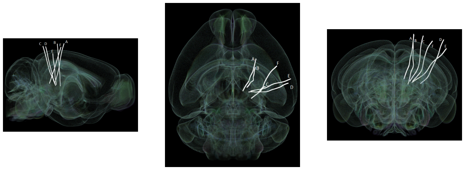
The images below were rendered using the Visualizing Neuropixels Probe Locations notebook. The probes are using the Common Coordinate Framework (CCF). The experiment uses six probes labeled A-F to target various regions.

sagittal_view = Image.open("../../data/images/probes_sagittal.png")
dorsal_view = Image.open("../../data/images/probes_dorsal.png")
transverse_view = Image.open("../../data/images/probes_transverse.png")
fig, axes = plt.subplots(1,3,figsize=(20,60))

axes[0].imshow(sagittal_view)
axes[1].imshow(dorsal_view)
axes[2].imshow(transverse_view)
for ax in axes:
    ax.axis("off")

Extracting Units Spikes

Below, the Units table is retrieved from the file. It contains many metrics for every putative neuronal unit, printed below. For the analysis in this notebook, we are only interested in the spike_times attribute. This is an array of timestamps that a spike is measured for each unit. For more information on the various unit metrics, see Visualizing Unit Quality Metrics. From this table, the Units used in this notebook are selected if they have ‘good’ quality rather than ‘noise’, and if they belong in one of the regions of the primary visual cortex.

units = nwb.units
units[:10]

	amplitude_cutoff	presence_ratio	waveform_duration	amplitude	silhouette_score	PT_ratio	recovery_slope	peak_channel_id	cumulative_drift	quality	...	local_index	snr	cluster_id	isolation_distance	spread	repolarization_slope	isi_violations	spike_times	spike_amplitudes	waveform_mean
id
18	0.482676	0.99	0.247236	172.961490	-1.000000	0.724197	-0.235438	1	375.54	good	...	0	2.370060	0	112.102182	40.0	0.771356	0.027914	[4.4922532152915045, 4.521086529276424, 5.1896...	[0.00018815992989274546, 0.0001718086339958319...	[[0.0, -0.19246499999999767, -0.79735499999999...
19	0.000096	0.99	0.302178	403.617240	0.160601	0.541992	-0.375900	2	224.26	good	...	1	4.747905	1	180.421246	30.0	1.717896	0.004550	[4.498786544240689, 4.510386536456586, 4.51451...	[0.0003950147274748102, 0.000379433914617874, ...	[[0.0, -0.8457149999999984, -1.123200000000004...
20	0.500000	0.99	0.206030	247.351065	0.056562	0.632188	-0.291355	2	254.41	good	...	2	2.428699	2	57.186741	40.0	1.077086	0.078133	[4.625819792329159, 4.695919745289025, 4.77635...	[0.00024276691510614911, 0.0002852838354924115...	[[0.0, 0.5785650000000002, 1.0783500000000057,...
21	0.500000	0.99	0.288442	233.452440	0.135265	0.542070	-0.225143	6	292.65	good	...	3	2.767570	3	74.723368	40.0	1.002852	0.094466	[5.500819205166296, 6.6461851032423676, 7.1312...	[0.00023846510196428897, 0.0002230177947947952...	[[0.0, 0.5621850000000004, 0.23263500000000126...
22	0.500000	0.69	0.260972	235.834170	0.063853	0.632228	-0.240738	6	55.66	noise	...	4	2.917154	4	64.444229	40.0	1.059915	0.937503	[4.510486536389482, 4.542219848428376, 4.57648...	[0.0001437588984811566, 0.00016230849080827827...	[[0.0, 0.28294499999999934, -0.242384999999991...
23	0.500000	0.99	0.274707	205.786035	0.145720	0.667836	-0.234488	9	276.18	good	...	5	3.011839	5	101.471939	50.0	0.951812	0.160858	[4.933852918958796, 5.099152808035343, 5.11218...	[0.00020715961295061512, 0.0002016031257275142...	[[0.0, 0.5955299999999992, 0.8347949999999995,...
24	0.049857	0.99	0.315913	199.134390	0.174509	0.746555	-0.199070	14	105.24	good	...	6	3.257283	6	311.816760	20.0	0.853772	0.012911	[4.79338634655134, 4.877719623293358, 5.149552...	[0.00016360321872699657, 0.0001515125492480918...	[[0.0, 1.270620000000001, 1.5272399999999986, ...
25	0.488095	0.99	0.741709	48.485775	0.136921	1.005407	-0.011557	15	828.80	good	...	7	0.748003	7	-1.000000	140.0	0.029073	3.962069	[5.673085756234575, 5.898452271670457, 6.99561...	[0.00010823618746646498, 0.0001112135220866243...	[[0.0, -0.5594549999999994, -1.833975000000002...
26	0.005778	0.99	0.260972	238.437420	0.141260	0.416539	-0.230931	80	280.85	noise	...	8	3.071278	8	-1.000000	20.0	1.055411	0.009034	[4.518086531289553, 4.541986515251619, 4.55781...	[0.00028906698408488974, 0.0002770941664859186...	[[0.0, -0.20494500000000304, -0.10919999999999...
27	0.500000	0.99	2.211390	76.297065	0.070798	0.455506	-0.713997	92	559.18	noise	...	9	0.845542	9	43.578645	170.0	0.022582	1.425694	[4.71968639600723, 4.74718637755354, 4.8371196...	[5.3298862561483384e-05, 5.0203306663503646e-0...	[[0.0, -0.37186499999999834, 0.344174999999995...

10 rows × 29 columns

# select electrodes
channel_probes = {}

electrodes = nwb.electrodes
for i in range(len(electrodes)):
    channel_id = electrodes["id"][i]
    location = electrodes["location"][i]
    channel_probes[channel_id] = location

# function aligns location information from electrodes table with channel id from the units table
def get_unit_location(row):
    return channel_probes[int(row.peak_channel_id)]

print(set(get_unit_location(row) for row in units))

{'VISp1', 'VISam1', 'LGd-sh', 'APN', 'SUB', 'NB', 'VISl4', 'SGN', 'VISpm4', 'CA3', 'POL', 'DG-po', 'VISl1', 'MRN', 'VISrl2/3', 'TH', 'VISl5', 'MB', 'VISpm5', 'VISrl6b', 'VISrl6a', 'VISp6b', 'VISrl4', 'VISp4', 'DG-mo', 'VISrl5', 'VISpm6b', 'VISam5', 'VISl6b', 'MGd', 'DG-sg', 'VISam6a', 'HPF', 'VISl2/3', 'MGm', 'VISam2/3', 'ProS', 'POST', 'CA1', 'VISp5', 'VISl6a', 'LP', 'VISpm6a', 'SCig', 'VISam4', 'VISpm2/3', 'VISp2/3', 'VISp6a', 'VISrl1', 'root', 'PoT'}

### selecting units spike times

brain_regions = ["VISp6a", "VISp5", "VISp4", "VISp6b", "VISp2/3"]

# select units based if they have 'good' quality and exists in one of the specified brain_regions
units_spike_times = []
for location in brain_regions:
    location_units_spike_times = []
    for row in units:
        if get_unit_location(row) == location and row.quality.item() == "good":
            location_units_spike_times.append(row.spike_times.item())
    units_spike_times += location_units_spike_times

print(len(units_spike_times))

175

Session Timeline

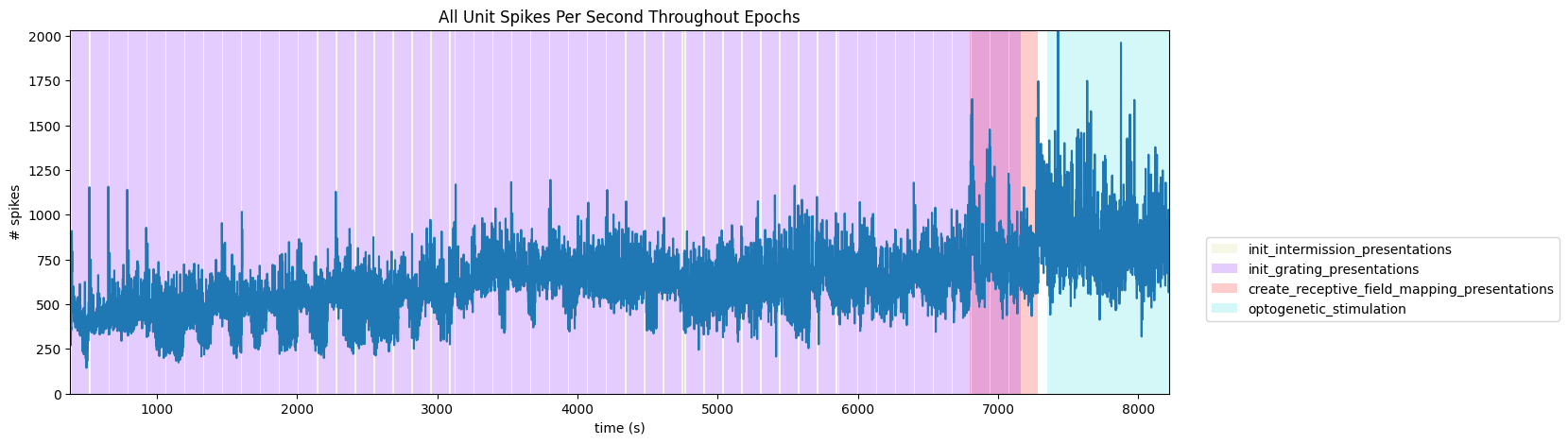
To get a good idea of the order and the way stimulus is shown throughout the session, the code below generates a timeline of the various ‘epochs’ of stimulus. It can be seen that there are many repeated epochs of the gratings presentation, interspersed with intermission presentations, followed by an epoch of receptive field presentations. Note that there is an overlap of two epochs, the final gratings and the receptive field mapping presentations. This is due to a unintended stim design mistake, please be careful when analyzing data from this period.

# extract epoch times from stim table where stimulus rows have a different 'block' than following row
# returns list of epochs, where an epoch is of the form (stimulus name, stimulus block, start time, stop time)
def extract_epochs(stim_name, stim_table, epochs):
    
    # specify a current epoch stop and start time
    epoch_start = stim_table.start_time[0]
    epoch_stop = stim_table.stop_time[0]

    # for each row, try to extend current epoch stop_time
    for i in range(len(stim_table)):
        this_block = stim_table.stimulus_block[i]
        # if end of table, end the current epoch
        if i+1 >= len(stim_table):
            epochs.append((stim_name, this_block, epoch_start, epoch_stop))
            break
            
        next_block = stim_table.stimulus_block[i+1]
        # if next row is the same stim block, push back epoch_stop time
        if next_block == this_block:
            epoch_stop = stim_table.stop_time[i+1]
        # otherwise, end the current epoch, start new epoch
        else:
            epochs.append((stim_name, this_block, epoch_start, epoch_stop))
            epoch_start = stim_table.start_time[i+1]
            epoch_stop = stim_table.stop_time[i+1]
    
    return epochs

# extract epochs from all valid stimulus tables
epochs = []
for stim_name in nwb.intervals.keys():
    stim_table = nwb.intervals[stim_name]
    try:
        epochs = extract_epochs(stim_name, stim_table, epochs)
    except:
        continue

# manually add optotagging epoch since the table is stored separately
opto_stim_table = nwb.processing["optotagging"]["optogenetic_stimulation"]
opto_epoch = ("optogenetic_stimulation", 1.0, opto_stim_table.start_time[0], opto_stim_table.stop_time[-1])
epochs.append(opto_epoch)

# epochs take the form (stimulus name, stimulus block, start time, stop time)
print(len(epochs))
epochs.sort(key=lambda x: x[2])
for epoch in epochs:
    print(epoch)

108
('init_intermission_presentations', 0.0, 381.69655, 391.70494)
('init_grating_presentations', 1.0, 391.70494, 516.30978)
('init_intermission_presentations', 2.0, 516.81017, 526.81866)
('init_grating_presentations', 3.0, 526.81866, 651.42343)
('init_intermission_presentations', 4.0, 651.92384, 661.93225)
('init_grating_presentations', 5.0, 661.93225, 786.53705)
('init_intermission_presentations', 6.0, 787.03745, 797.0459)
('init_grating_presentations', 7.0, 797.0459, 921.6507)
('init_intermission_presentations', 8.0, 922.15112, 932.15956)
('init_grating_presentations', 9.0, 932.15956, 1056.76434)
('init_intermission_presentations', 10.0, 1057.26479, 1067.27318)
('init_grating_presentations', 11.0, 1067.27318, 1191.87797)
('init_intermission_presentations', 12.0, 1192.3784, 1202.38679)
('init_grating_presentations', 13.0, 1202.38679, 1326.99161)
('init_intermission_presentations', 14.0, 1327.49204, 1337.50046)
('init_grating_presentations', 15.0, 1337.50046, 1462.10523)
('init_intermission_presentations', 16.0, 1462.60567, 1472.61419)
('init_grating_presentations', 17.0, 1472.61419, 1597.21887)
('init_intermission_presentations', 18.0, 1597.7193, 1607.72771)
('init_grating_presentations', 19.0, 1607.72771, 1732.33249)
('init_intermission_presentations', 20.0, 1732.83289, 1742.84133)
('init_grating_presentations', 21.0, 1742.84133, 1867.44613)
('init_intermission_presentations', 22.0, 1867.94656, 1877.95497)
('init_grating_presentations', 23.0, 1877.95497, 2002.55975)
('init_intermission_presentations', 24.0, 2003.06018, 2013.06859)
('init_grating_presentations', 25.0, 2013.06859, 2139.5583)
('init_intermission_presentations', 26.0, 2140.05873, 2150.06711)
('init_grating_presentations', 27.0, 2150.06711, 2274.67192)
('init_intermission_presentations', 28.0, 2275.17236, 2285.18077)
('init_grating_presentations', 29.0, 2285.18077, 2409.78556)
('init_intermission_presentations', 30.0, 2410.28599, 2420.2944)
('init_grating_presentations', 31.0, 2420.2944, 2544.89923)
('init_intermission_presentations', 32.0, 2545.39962, 2555.40806)
('init_grating_presentations', 33.0, 2555.40806, 2680.01283)
('init_intermission_presentations', 34.0, 2680.51324, 2690.52167)
('init_grating_presentations', 35.0, 2690.52167, 2815.12647)
('init_intermission_presentations', 36.0, 2815.62691, 2825.63528)
('init_grating_presentations', 37.0, 2825.63528, 2950.24009)
('init_intermission_presentations', 38.0, 2950.74053, 2960.74894)
('init_grating_presentations', 39.0, 2960.74894, 3085.35374)
('init_intermission_presentations', 40.0, 3085.85414, 3095.86259)
('init_grating_presentations', 41.0, 3095.86259, 3120.3832)
('init_intermission_presentations', 42.0, 3120.88362, 3130.89201)
('init_grating_presentations', 43.0, 3130.89201, 3255.49683)
('init_intermission_presentations', 44.0, 3255.99729, 3266.00567)
('init_grating_presentations', 45.0, 3266.00567, 3390.61046)
('init_intermission_presentations', 46.0, 3391.1109, 3401.11938)
('init_grating_presentations', 47.0, 3401.11938, 3525.72409)
('init_intermission_presentations', 48.0, 3526.22452, 3536.23294)
('init_grating_presentations', 49.0, 3536.23294, 3660.83773)
('init_intermission_presentations', 50.0, 3661.33813, 3671.34658)
('init_grating_presentations', 51.0, 3671.34658, 3795.95137)
('init_intermission_presentations', 52.0, 3796.4518, 3806.46022)
('init_grating_presentations', 53.0, 3806.46022, 3931.06501)
('init_intermission_presentations', 54.0, 3931.56544, 3941.57382)
('init_grating_presentations', 55.0, 3941.57382, 4066.17863)
('init_intermission_presentations', 56.0, 4066.67907, 4076.68749)
('init_grating_presentations', 57.0, 4076.68749, 4201.29228)
('init_intermission_presentations', 58.0, 4201.79269, 4211.80112)
('init_grating_presentations', 59.0, 4211.80112, 4336.40592)
('init_intermission_presentations', 60.0, 4336.90635, 4346.91476)
('init_grating_presentations', 61.0, 4346.91476, 4471.51956)
('init_intermission_presentations', 62.0, 4472.01996, 4482.0284)
('init_grating_presentations', 63.0, 4482.0284, 4606.6332)
('init_intermission_presentations', 64.0, 4607.13359, 4617.14205)
('init_grating_presentations', 65.0, 4617.14205, 4741.74684)
('init_intermission_presentations', 66.0, 4742.24727, 4752.25568)
('init_grating_presentations', 67.0, 4752.25568, 4761.7637)
('init_intermission_presentations', 68.0, 4762.2641, 4772.27252)
('init_grating_presentations', 69.0, 4772.27252, 4896.87731)
('init_intermission_presentations', 70.0, 4897.37774, 4907.38619)
('init_grating_presentations', 71.0, 4907.38619, 5031.99096)
('init_intermission_presentations', 72.0, 5032.49138, 5042.4998)
('init_grating_presentations', 73.0, 5042.4998, 5167.10456)
('init_intermission_presentations', 74.0, 5167.60502, 5177.61349)
('init_grating_presentations', 75.0, 5177.61349, 5302.21821)
('init_intermission_presentations', 76.0, 5302.71863, 5312.72708)
('init_grating_presentations', 77.0, 5312.72708, 5437.33184)
('init_intermission_presentations', 78.0, 5437.83228, 5447.84072)
('init_grating_presentations', 79.0, 5447.84072, 5572.44554)
('init_intermission_presentations', 80.0, 5572.94596, 5582.95439)
('init_grating_presentations', 81.0, 5582.95439, 5707.55911)
('init_intermission_presentations', 82.0, 5708.0596, 5718.06809)
('init_grating_presentations', 83.0, 5718.06809, 5842.67278)
('init_intermission_presentations', 84.0, 5843.17322, 5853.18163)
('init_grating_presentations', 85.0, 5853.18163, 5857.6854)
('init_intermission_presentations', 86.0, 5858.18584, 5868.19423)
('init_grating_presentations', 87.0, 5868.19423, 5992.79906)
('init_intermission_presentations', 88.0, 5993.29951, 6003.30787)
('init_grating_presentations', 89.0, 6003.30787, 6127.91269)
('init_intermission_presentations', 90.0, 6128.41312, 6138.42155)
('init_grating_presentations', 91.0, 6138.42155, 6263.02633)
('init_intermission_presentations', 92.0, 6263.52676, 6273.53515)
('init_grating_presentations', 93.0, 6273.53515, 6398.13998)
('init_intermission_presentations', 94.0, 6398.64041, 6408.64884)
('init_grating_presentations', 95.0, 6408.64884, 6533.25366)
('init_intermission_presentations', 96.0, 6533.75403, 6543.76247)
('init_grating_presentations', 97.0, 6543.76247, 6668.36726)
('init_intermission_presentations', 98.0, 6668.86769, 6678.87611)
('init_grating_presentations', 99.0, 6678.87611, 6803.48092)
('create_receptive_field_mapping_presentations', 100.0, 6794.97378, 7281.38293)
('init_intermission_presentations', 101.0, 6803.98131, 6813.98979)
('init_grating_presentations', 102.0, 6813.98979, 6938.59456)
('init_intermission_presentations', 103.0, 6939.09498, 6949.1034)
('init_grating_presentations', 104.0, 6949.1034, 7073.70817)
('init_intermission_presentations', 105.0, 7074.20862, 7084.21703)
('init_grating_presentations', 106.0, 7084.21703, 7158.77976)
('optogenetic_stimulation', 1.0, 7353.87906, 8219.60458)

time_start = floor(min([epoch[2] for epoch in epochs]))
time_end = ceil(max([epoch[3] for epoch in epochs]))
all_units_spike_times = np.concatenate(units_spike_times).ravel()
print(time_start, time_end)

# make histogram of unit spikes per second over specified timeframe
time_bin_edges = np.linspace(time_start, time_end, (time_end-time_start))
hist, bins = np.histogram(all_units_spike_times, bins=time_bin_edges)

381 8220

# generate plot of spike histogram with colored epoch intervals and legend
fig, ax = plt.subplots(figsize=(15,5))

# assign unique color to each stimulus name
stim_names = list({epoch[0] for epoch in epochs})
colors = plt.cm.rainbow(np.linspace(0,1,len(stim_names)))
stim_color_map = {stim_names[i]:colors[i] for i in range(len(stim_names))}

epoch_key = {}
height = max(hist)
# draw colored rectangles for each epoch
for epoch in epochs:
    stim_name, stim_block, epoch_start, epoch_end = epoch
    color = stim_color_map[stim_name]
    rec = ax.add_patch(mpl.patches.Rectangle((epoch_start, 0), epoch_end-epoch_start, height, alpha=0.2, facecolor=color))
    epoch_key[stim_name] = rec

ax.set_xlim(time_start, time_end)
ax.set_ylim(-0.1, height+0.1)
ax.set_xlabel("time (s)")
ax.set_ylabel("# spikes")
ax.set_title("All Unit Spikes Per Second Throughout Epochs")

fig.legend(epoch_key.values(), epoch_key.keys(), loc="lower right", bbox_to_anchor=(1.18, 0.25))
ax.plot(bins[:-1], hist)

[<matplotlib.lines.Line2D at 0x198da70e380>]

Extracting Stimulus Times

nwb.intervals.keys()

dict_keys(['create_receptive_field_mapping_presentations', 'init_grating_presentations', 'init_intermission_presentations', 'invalid_times', 'spontaneous_presentations'])

stim_table = nwb.intervals["init_grating_presentations"]
print(np.mean(np.diff(stim_table.start_time)))
print({elem for elem in stim_table.orientation if not np.isnan(elem)})

1.0845607324891808
{45.0, 135.0}

stim_table[:10]

	start_time	stop_time	stimulus_name	stimulus_block	contrast	temporal_frequency	spatial_frequency	orientation	color	mask	opacity	size	units	stimulus_index	phase	tags	timeseries
id
0	391.70494	392.20535	init_grating	1.0	0.8	4.0	0.04	135.0	[1.0, 1.0, 1.0]	None	1.0	[1000.0, 1000.0]	deg	1.0	0.0	[stimulus_time_interval]	[(2, 1, timestamps pynwb.base.TimeSeries at 0x...
1	392.70578	393.20620	init_grating	1.0	0.8	4.0	0.04	135.0	[1.0, 1.0, 1.0]	None	1.0	[1000.0, 1000.0]	deg	1.0	0.0	[stimulus_time_interval]	[(3, 1, timestamps pynwb.base.TimeSeries at 0x...
2	393.70662	394.20704	init_grating	1.0	0.8	4.0	0.04	135.0	[1.0, 1.0, 1.0]	None	1.0	[1000.0, 1000.0]	deg	1.0	0.0	[stimulus_time_interval]	[(4, 1, timestamps pynwb.base.TimeSeries at 0x...
3	394.70747	395.20789	init_grating	1.0	0.8	4.0	0.04	45.0	[1.0, 1.0, 1.0]	None	1.0	[1000.0, 1000.0]	deg	1.0	0.0	[stimulus_time_interval]	[(5, 1, timestamps pynwb.base.TimeSeries at 0x...
4	395.70831	396.20873	init_grating	1.0	NaN	NaN	NaN	NaN	[1.0, 1.0, 1.0]	None	1.0	[1000.0, 1000.0]	deg	1.0	N/A	[stimulus_time_interval]	[(6, 1, timestamps pynwb.base.TimeSeries at 0x...
5	396.70915	397.20955	init_grating	1.0	0.8	4.0	0.04	135.0	[1.0, 1.0, 1.0]	None	1.0	[1000.0, 1000.0]	deg	1.0	0.0	[stimulus_time_interval]	[(7, 1, timestamps pynwb.base.TimeSeries at 0x...
6	397.71003	398.21042	init_grating	1.0	0.8	4.0	0.04	135.0	[1.0, 1.0, 1.0]	None	1.0	[1000.0, 1000.0]	deg	1.0	0.0	[stimulus_time_interval]	[(8, 1, timestamps pynwb.base.TimeSeries at 0x...
7	398.71085	399.21128	init_grating	1.0	0.8	4.0	0.04	135.0	[1.0, 1.0, 1.0]	None	1.0	[1000.0, 1000.0]	deg	1.0	0.0	[stimulus_time_interval]	[(9, 1, timestamps pynwb.base.TimeSeries at 0x...
8	399.71168	400.21214	init_grating	1.0	0.8	4.0	0.04	45.0	[1.0, 1.0, 1.0]	None	1.0	[1000.0, 1000.0]	deg	1.0	0.0	[stimulus_time_interval]	[(10, 1, timestamps pynwb.base.TimeSeries at 0...
9	400.71252	401.21294	init_grating	1.0	NaN	NaN	NaN	NaN	[1.0, 1.0, 1.0]	None	1.0	[1000.0, 1000.0]	deg	1.0	N/A	[stimulus_time_interval]	[(11, 1, timestamps pynwb.base.TimeSeries at 0...

# select times where there is a local oddball
lo_stim_select = lambda prev_row, row, next_row: prev_row.orientation.item() == 135.0 and row.orientation.item() == 45.0 and np.isnan(next_row.orientation.item())
lo_stim_times = [float(stim_table[i].start_time) for i in range(1,len(stim_table)-1) if lo_stim_select(stim_table[i-1], stim_table[i], stim_table[i+1])]
print(len(lo_stim_times))

# select times where there is a global oddball
go_stim_select = lambda prev_row, row, next_row: prev_row.orientation.item() == 135.0 and row.orientation.item() == 135.0 and np.isnan(next_row.orientation.item())
go_stim_times = [float(stim_table[i].start_time) for i in range(1,len(stim_table)-1) if go_stim_select(stim_table[i-1], stim_table[i], stim_table[i+1])]
print(len(go_stim_times))

675
322

Generating Spike Matrix

# bin size for counting spikes
time_resolution = 0.005

# start and end times (relative to the stimulus at 0 seconds) that we want to examine and align spikes to
window_start_time = -0.25
window_end_time = 0.5

def get_spike_matrix(stim_times, units_spike_times, bin_edges):
    time_resolution = np.mean(np.diff(bin_edges))
    # 3D spike matrix to be populated with spike counts
    spike_matrix = np.zeros((len(units_spike_times), len(stim_times), len(bin_edges)-1))

    # populate 3D spike matrix for each unit for each stimulus trial by counting spikes into bins
    for unit_idx in range(len(units_spike_times)):
        spike_times = units_spike_times[unit_idx]

        for stim_idx, stim_time in enumerate(stim_times):
            # get spike times that fall within the bin's time range relative to the stim time        
            first_bin_time = stim_time + bin_edges[0]
            last_bin_time = stim_time + bin_edges[-1]
            first_spike_in_range, last_spike_in_range = np.searchsorted(spike_times, [first_bin_time, last_bin_time])
            spike_times_in_range = spike_times[first_spike_in_range:last_spike_in_range]

            # convert spike times into relative time bin indices
            bin_indices = ((spike_times_in_range - (first_bin_time)) / time_resolution).astype(int)
            
            # mark that there is a spike at these bin times for this unit on this stim trial
            for bin_idx in bin_indices:
                spike_matrix[unit_idx, stim_idx, bin_idx] += 1

    return spike_matrix

# time bins used
n_bins = int((window_end_time - window_start_time) / time_resolution)
bin_edges = np.linspace(window_start_time, window_end_time, n_bins, endpoint=True)

# calculate baseline and stimulus interval indices for use later
stimulus_onset_idx = int(-bin_edges[0] / time_resolution)

lo_spike_matrix = get_spike_matrix(lo_stim_times, units_spike_times, bin_edges)
go_spike_matrix = get_spike_matrix(go_stim_times, units_spike_times, bin_edges)

print(lo_spike_matrix.shape)
print(go_spike_matrix.shape)

(175, 675, 149)
(175, 322, 149)

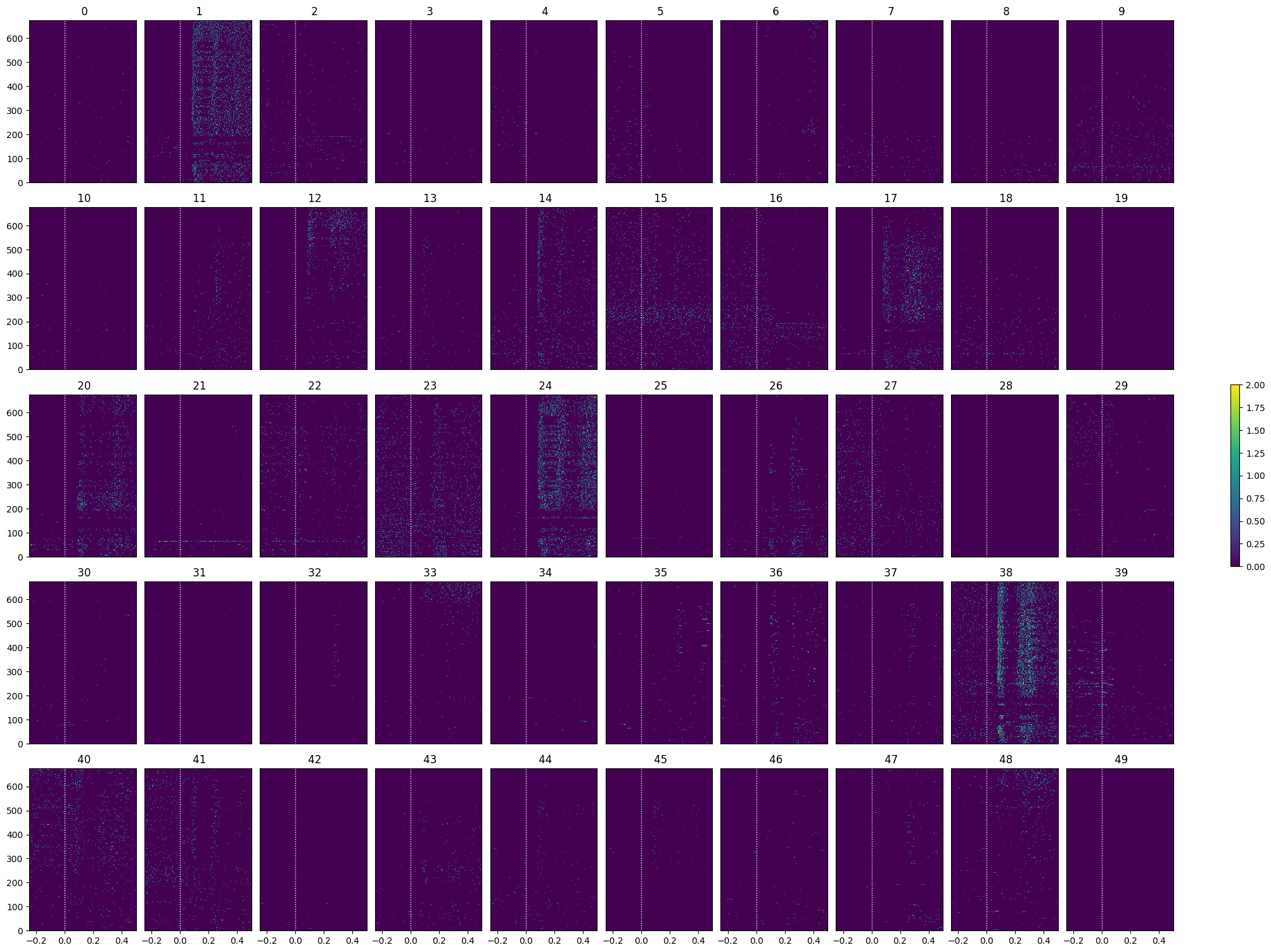
Showing Response Windows

After generating spike matrices, we can view the PSTHs for each unit.

def show_response(ax, window, window_start_time, window_end_time, aspect="auto", vmin=None, vmax=None, yticklabels=[], skipticks=1, xlabel="Time (s)", ylabel="ROI", cbar=True, cbar_label=None):
    if len(window) == 0:
        print("Input data has length 0; Nothing to display")
        return

    img = ax.imshow(window, aspect=aspect, extent=[window_start_time, window_end_time, 0, len(window)], interpolation="none", vmin=vmin, vmax=vmax)
    if cbar:
        ax.colorbar(img, shrink=0.5, label=cbar_label)

    ax.plot([0,0],[0, len(window)], ":", color="white", linewidth=1.0)

    if len(yticklabels) != 0:
        ax.set_yticks(range(len(yticklabels)))
        ax.set_yticklabels(yticklabels, fontsize=8)

        n_ticks = len(yticklabels[::skipticks])
        ax.yaxis.set_major_locator(plt.MaxNLocator(n_ticks))

    ax.set_xlabel(xlabel)
    ax.set_ylabel(ylabel)

def show_many_responses(windows, rows, cols, window_idxs=None, title=None, subplot_title="", xlabel=None, ylabel=None, cbar_label=None, vmin=0, vmax=2):
    if window_idxs is None:
        window_idxs = range(len(windows))
    windows = windows[window_idxs]
    
    # handle case with no input data
    if len(windows) == 0:
        print("Input data has length 0; Nothing to display")
        return
    # handle cases when there aren't enough windows for number of rows
    if len(windows) < rows*cols:
        rows = (len(windows) // cols) + 1

    fig, axes = plt.subplots(rows, cols, figsize=(2*cols, 3*rows), layout="constrained")
    # handle case when there's only one row
    if len(axes.shape) == 1:
        axes = axes.reshape((1, axes.shape[0]))

    for i in range(rows*cols):
        ax_row = int(i // cols)
        ax_col = i % cols
        ax = axes[ax_row][ax_col]
        
        if i > len(windows)-1:
            ax.set_visible(False)
            continue

        window = windows[i]
        show_response(ax, window, window_start_time, window_end_time, xlabel=xlabel, ylabel=ylabel, cbar=False, vmin=vmin, vmax=vmax)
        ax.set_title(f"{subplot_title} {window_idxs[i]}")
        if ax_row != rows-1:
            ax.get_xaxis().set_visible(False)
        if ax_col != 0:
            ax.get_yaxis().set_visible(False)

    fig.suptitle(title)
    norm = mpl.colors.Normalize(vmin=vmin, vmax=vmax)
    colorbar = fig.colorbar(mpl.cm.ScalarMappable(norm=norm), ax=axes, shrink=2/cols, label=cbar_label)

show_many_responses(lo_spike_matrix, 5, 10)

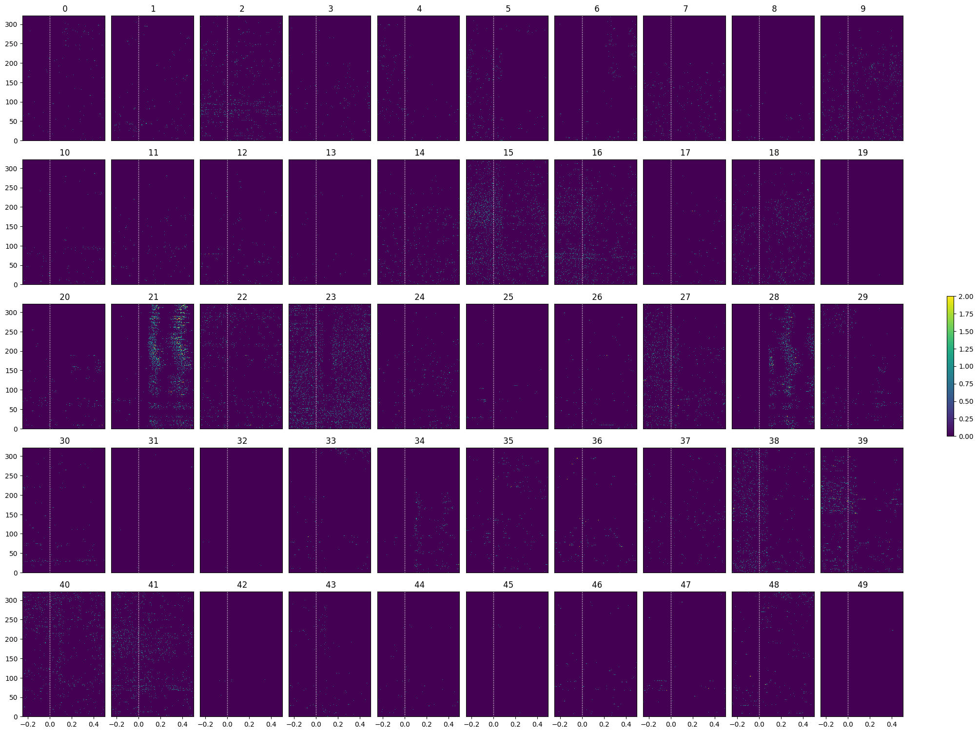
show_many_responses(go_spike_matrix, 5, 10)

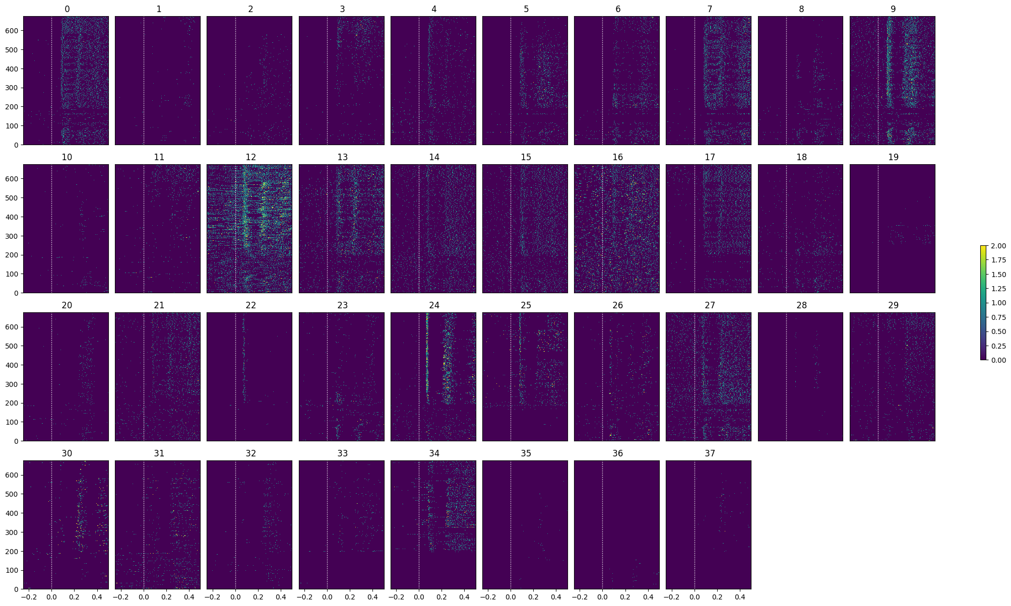
Selecting Responsive Cells

As discussed in Statistically Testing 2P Responses to Stimulus, the criteria used to select for responsive cells can have a significant impact. Here, the simple criterion is to select units whose post-stimulus z-scores are greater than 1 or less than -1.

def select_cells(spike_matrix, stimulus_onset_idx):
    baseline_means = np.mean(spike_matrix[:,:,:stimulus_onset_idx], axis=2)
    mean_baseline_means = np.mean(baseline_means, axis=1)
    std_baseline_means = np.std(baseline_means, axis=1)

    response_means = np.mean(spike_matrix[:,:,stimulus_onset_idx:], axis=2)
    mean_response_means = np.mean(response_means, axis=1)

    unit_z_scores = (mean_response_means - mean_baseline_means) / std_baseline_means
    return np.where(np.logical_or(unit_z_scores > 1, unit_z_scores < -1))[0]

lo_selected_idxs = select_cells(lo_spike_matrix, stimulus_onset_idx)
show_many_responses(lo_spike_matrix[lo_selected_idxs], 5, 10)

go_selected_idxs = select_cells(go_spike_matrix, stimulus_onset_idx)
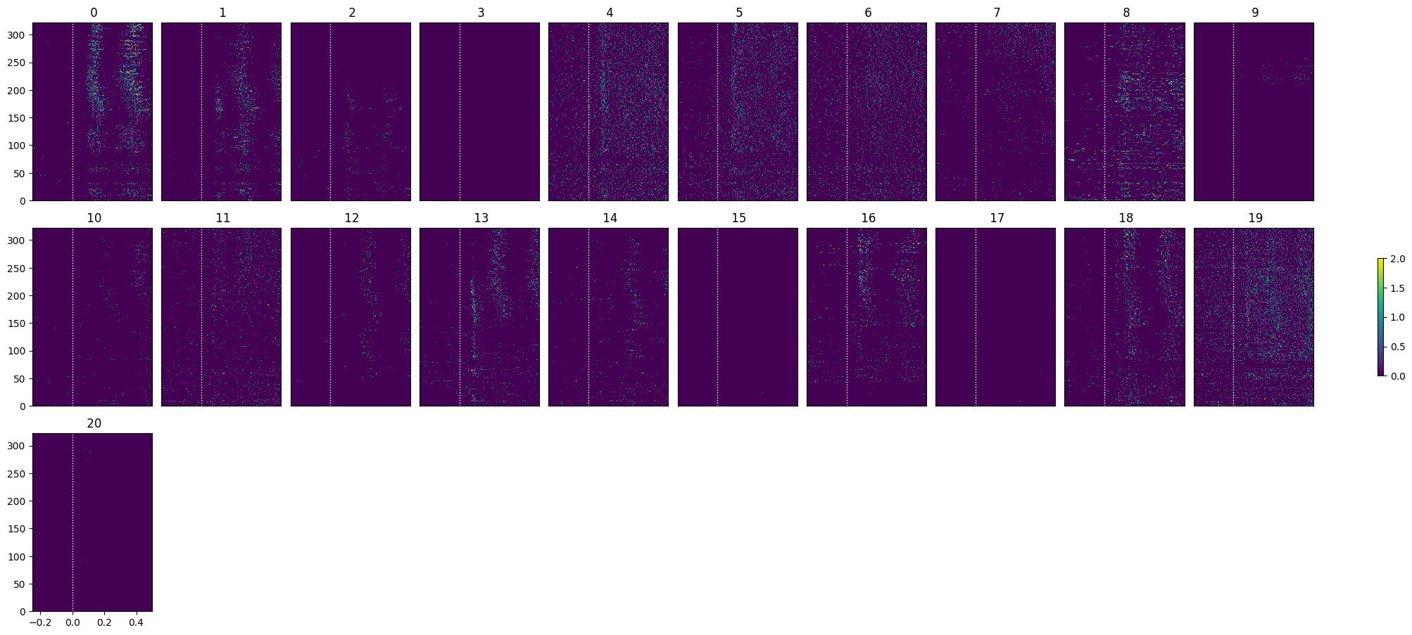
show_many_responses(go_spike_matrix[go_selected_idxs], 5, 10)

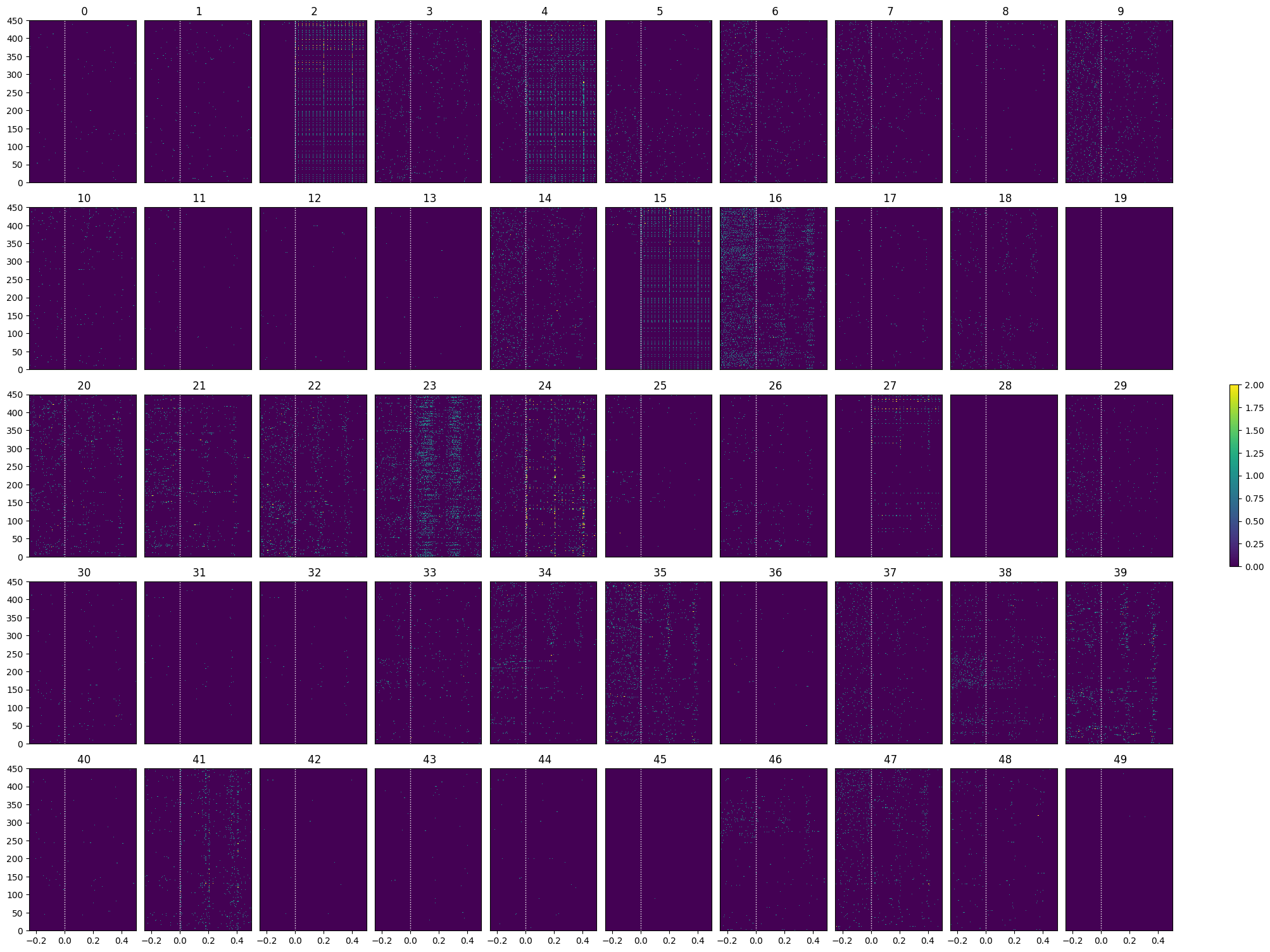
Optotagging

As mentioned earlier, the final epoch of the sessions is optotagging. The principles behind the optotagging are discussed in the Identifying Optotagged Units notebook.

opto_stim_table = nwb.processing["optotagging"]["optogenetic_stimulation"]
opto_stim_table[:20]

	start_time	condition	level	stop_time	stimulus_name	duration	tags	timeseries
id
0	7353.87906	Each pulse is 10 ms wide	0.77	7354.87906	5 hz pulse train	1.0	[optical_stimulation]	[(0, 1, optotagging pynwb.ogen.OptogeneticSeri...
1	7355.69162	Each pulse is 6 ms wide	0.77	7356.69162	40 hz pulse train	1.0	[optical_stimulation]	[(1, 1, optotagging pynwb.ogen.OptogeneticSeri...
2	7357.78428	half-period of a cosine wave	0.97	7358.78428	raised_cosine	1.0	[optical_stimulation]	[(2, 1, optotagging pynwb.ogen.OptogeneticSeri...
3	7359.49488	Each pulse is 6 ms wide	0.97	7360.49488	40 hz pulse train	1.0	[optical_stimulation]	[(3, 1, optotagging pynwb.ogen.OptogeneticSeri...
4	7361.26577	Each pulse is 6 ms wide	0.77	7362.26577	40 hz pulse train	1.0	[optical_stimulation]	[(4, 1, optotagging pynwb.ogen.OptogeneticSeri...
5	7363.29037	Each pulse is 10 ms wide	0.77	7364.29037	5 hz pulse train	1.0	[optical_stimulation]	[(5, 1, optotagging pynwb.ogen.OptogeneticSeri...
6	7365.33388	Each pulse is 6 ms wide	0.77	7366.33388	40 hz pulse train	1.0	[optical_stimulation]	[(6, 1, optotagging pynwb.ogen.OptogeneticSeri...
7	7367.06362	Each pulse is 10 ms wide	0.97	7368.06362	5 hz pulse train	1.0	[optical_stimulation]	[(7, 1, optotagging pynwb.ogen.OptogeneticSeri...
8	7368.86419	Each pulse is 10 ms wide	0.77	7369.86419	5 hz pulse train	1.0	[optical_stimulation]	[(8, 1, optotagging pynwb.ogen.OptogeneticSeri...
9	7370.97949	Each pulse is 10 ms wide	0.77	7371.97949	5 hz pulse train	1.0	[optical_stimulation]	[(9, 1, optotagging pynwb.ogen.OptogeneticSeri...
10	7372.75026	Each pulse is 10 ms wide	0.77	7373.75026	5 hz pulse train	1.0	[optical_stimulation]	[(10, 1, optotagging pynwb.ogen.OptogeneticSer...
11	7374.69303	Each pulse is 6 ms wide	0.97	7375.69303	40 hz pulse train	1.0	[optical_stimulation]	[(11, 1, optotagging pynwb.ogen.OptogeneticSer...
12	7376.85340	Each pulse is 10 ms wide	1.35	7377.85340	5 hz pulse train	1.0	[optical_stimulation]	[(12, 1, optotagging pynwb.ogen.OptogeneticSer...
13	7378.94733	half-period of a cosine wave	0.97	7379.94733	raised_cosine	1.0	[optical_stimulation]	[(13, 1, optotagging pynwb.ogen.OptogeneticSer...
14	7380.66683	Each pulse is 6 ms wide	0.97	7381.66683	40 hz pulse train	1.0	[optical_stimulation]	[(14, 1, optotagging pynwb.ogen.OptogeneticSer...
15	7382.51879	half-period of a cosine wave	0.97	7383.51879	raised_cosine	1.0	[optical_stimulation]	[(15, 1, optotagging pynwb.ogen.OptogeneticSer...
16	7384.50218	Each pulse is 6 ms wide	1.35	7385.50218	40 hz pulse train	1.0	[optical_stimulation]	[(16, 1, optotagging pynwb.ogen.OptogeneticSer...
17	7386.66661	half-period of a cosine wave	1.35	7387.66661	raised_cosine	1.0	[optical_stimulation]	[(17, 1, optotagging pynwb.ogen.OptogeneticSer...
18	7388.82201	Each pulse is 10 ms wide	0.77	7389.82201	5 hz pulse train	1.0	[optical_stimulation]	[(18, 1, optotagging pynwb.ogen.OptogeneticSer...
19	7390.86515	half-period of a cosine wave	0.77	7391.86515	raised_cosine	1.0	[optical_stimulation]	[(19, 1, optotagging pynwb.ogen.OptogeneticSer...

opto_stim_times = [float(row.start_time) for row in opto_stim_table if isclose(float(row.duration), 1.0)]
len(opto_stim_times)
len(units_spike_times)

175

# bin size for counting spikes
time_resolution = 0.005

# start and end times (relative to the stimulus at 0 seconds) that we want to examine and align spikes to
window_start_time = -0.25
window_end_time = 0.5

# time bins used
n_bins = int((window_end_time - window_start_time) / time_resolution)
bin_edges = np.linspace(window_start_time, window_end_time, n_bins, endpoint=True)

# calculate baseline and stimulus interval indices for use later
stimulus_onset_idx = int(-bin_edges[0] / time_resolution)

opto_spike_matrix = get_spike_matrix(opto_stim_times, units_spike_times, bin_edges)

print(opto_spike_matrix.shape)

(175, 450, 149)

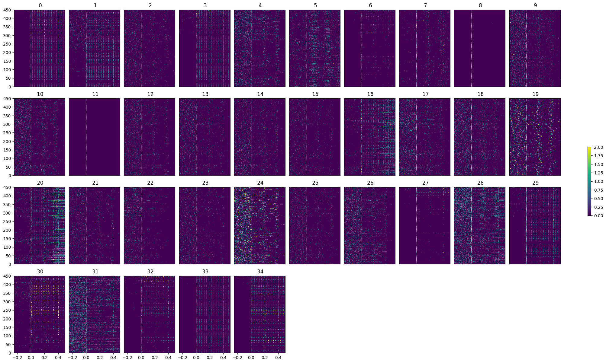
show_many_responses(opto_spike_matrix, 5, 10)

opto_selected_idxs = select_cells(opto_spike_matrix, stimulus_onset_idx)
show_many_responses(opto_spike_matrix[opto_selected_idxs], 5, 10)