OpenScope’s Vision2Hippocampus Dataset#
Introduction#
Extensive research shows that visual cortical neurons respond to specific stimuli, e.g. the primary visual cortical neurons respond to bars of light with specific orientation. In contrast, the hippocampal neurons are thought to encode not specific stimuli but instead represent abstract concepts such as space, time and events. How does this happen? Specifically, how does the representation of simple visual stimuli evolve from the thalamus, which is a synapse away from the retina, through primary visual cortex, higher order visual areas and all the way to hippocampus, that is farthest removed from the retina? That is the primary goal of this OpenScope project. We note that while visual cortical responses are commonly measured in stationary animals, with precise stimulus and behavioral control; hippocampal responses are measured in freely behaving rats where multisensory stimuli and multimodal behaviors contribute, but they are difficult to measure or controlled. Hence, recent research has pivoted to measuring hippocampal responses in virtual realty (VR)1–4. Although it was believed that hippocampal place cells in VR are similar to those in the real world, a careful and direct comparison showed that this is not the case5. In fact, contrary to common beliefs, when the multisensory and multimodal stimuli commonly present in the real world are eliminated in VR, these experiments revealed that vision and locomotion alone are not sufficient to generate hippocampal spatial selectivity6. Further, hippocampal neurons showed clear direction selectivity that was directly controlled by visual cues in VR7. Thus, elimination of nonspecific cues using VR revealed a growing similarity between hippocampal and visual cortical response to specific stimuli and that were behaviorally relevant8. To further confirm the sensory origins of hippocampal responses, subsequent experiments eliminated any specific behaviors, e.g. rewards, memory, navigation etc. and measured hippocampal responses in body- or head-fixed rodents to reveal strong selectivity to a moving bar of light9 with naso-temporal magnification commonly seen in V1. Further, careful analysis of prior OpenScope data from Allen Institute revealed that a black-and-white silent movie generated robust responses in the hippocampus that were related to the simultaneously measured visual cortical ones10.
Experiment design#
Two main categories of visual stimuli were presented–
Simple visual motion, elicited by basic stimuli, like bars of light.
Complex stimuli
Among each class, the following variants were used – Simple bars of light –
Vertical bar, moving left right (naso-temporal)
Horizontal bar, moving up and down and other variants
Complex visual stimuli – A 20 second clip of an eagle swooping down was used as the central “natural movie”, which was shown to all mice in the dataset. In 5 mice, another “natural movie” involving squirrels was used along with the eagle movie.
Examples of movies presented#
a) Simple stimuli : 
b) Complex stimuli : 
References#
Holscher, C. et al. Rats are able to navigate in virtual environments. The Journal of experimental biology 208, 561–9 (2005).
Harvey, C. D., Collman, F., Dombeck, D. A. & Tank, D. W. Intracellular dynamics of hippocampal place cells during virtual navigation. Nature 461, 941–946 (2009).
Chen, G., King, J. a, Burgess, N. & O’Keefe, J. How vision and movement combine in the hippocampal place code. Proc Natl Acad Sci U S A 110, 378–383 (2013).
Cushman, J. D. et al. Multisensory Control of Multimodal Behavior: Do the Legs Know What the Tongue Is Doing? PLoS ONE 8, e80465 (2013).
Ravassard, P. et al. Multisensory control of hippocampal spatiotemporal selectivity. Science (New York, N.Y.) 340, 1342–6 (2013).
Aghajan, Z. M. et al. Impaired spatial selectivity and intact phase precession in two-dimensional virtual reality. Nature neuroscience 18, 121–128 (2015).
Acharya, L., Aghajan, Z. M., Vuong, C., Moore, J. J. & Mehta, M. R. Causal Influence of Visual Cues on Hippocampal Directional Selectivity. Cell 164, 197–207 (2016).
Moore, J. J., Cushman, J. D., Acharya, L., Popeney, B. & Mehta, M. R. Linking hippocampal multiplexed tuning, Hebbian plasticity and navigation. Nature (2021) doi:10.1038/s41586-021-03989-z.
Purandare, C. S. et al. Moving bar of light evokes vectorial spatial selectivity in the immobile rat hippocampus. doi:10.1038/s41586-022-04404-x.
Purandare, C. & Mehta, M. Mega-scale movie-fields in the mouse visuo-hippocampal network. eLife 12, RP85069 (2023).
Environment Setup#
⚠️Note: If running on a new environment, run this cell once and then restart the kernel⚠️
try:
    from databook_utils.dandi_utils import dandi_download_open
except:
    !git clone https://github.com/AllenInstitute/openscope_databook.git
    %cd openscope_databook
    %pip install -e .
    %cd docs/projects
import os

import matplotlib as mpl
import matplotlib.pyplot as plt
import numpy as np
import pandas as pd

from math import floor, ceil, isclose
from PIL import Image
The Experiment#
session_files = pd.read_csv("../../data/vippo_sessions.csv")
session_files
| identifier | size | path | session_time | sub_name | sub_sex | sub_age | sub_genotype | probes | stim types | #_units | session_length | |
|---|---|---|---|---|---|---|---|---|---|---|---|---|
| 0 | 8ae65111-a130-47fc-a108-55e695374739 | 2448964467 | sub-692077/sub-692077_ses-1300222049.nwb | 2023-09-28 00:00:00-07:00 | 692077 | F | 89 | wt/wt | {'probeB', 'probeC', 'probeF', 'probeE', 'prob... | {'acurl_Wd15_Vel2_Bndry1_Cntst0_oneway_present... | 3091 | 7152.145567 |
| 1 | d3cfc0e4-eaa6-4cc0-b1de-9ed257cf0009 | 2237699442 | sub-695435/sub-695435_ses-1309235849.nwb | 2023-11-07 00:00:00-08:00 | 695435 | M | 109 | wt/wt | {'probeB', 'probeF', 'probeA', 'probeD'} | {'acurl_Wd15_Vel2_Bndry1_Cntst0_oneway_present... | 2251 | 7174.624310 |
| 2 | 24c71323-0446-4a06-83fa-f62ae21aba3e | 2457471091 | sub-715811/sub-715811_ses-1328842209.nwb | 2024-02-06 00:00:00-08:00 | 715811 | F | 106 | wt/wt | {'probeD', 'probeB', 'probeC', 'probeF', 'prob... | {'Stim04_SAC_Wd15_Vel2_Black_loop_presentation... | 2239 | 8117.399747 |
| 3 | 72e60080-722f-47f1-b8c0-91f9be1d5ef6 | 3073270590 | sub-702134/sub-702134_ses-1324803287.nwb | 2024-01-18 00:00:00-08:00 | 702134 | F | 135 | wt/wt | {'probeB', 'probeF', 'probeA', 'probeD'} | {'Stim04_SAC_Wd15_Vel2_Black_loop_presentation... | 3477 | 8124.426097 |
| 4 | 9b14e3b4-5d3e-4121-ae5e-ced7bc92af4e | 2892209972 | sub-702135/sub-702135_ses-1324561527.nwb | 2024-01-17 00:00:00-08:00 | 702135 | F | 134 | wt/wt | {'probeD', 'probeB', 'probeC', 'probeF', 'prob... | {'Stim04_SAC_Wd15_Vel2_Black_loop_presentation... | 2960 | 8125.099337 |
| 5 | 9b1bed43-3edf-40f9-a172-eb4c33883166 | 2923746400 | sub-714614/sub-714614_ses-1327183358.nwb | 2024-01-30 00:00:00-08:00 | 714614 | F | 106 | wt/wt | {'probeD', 'probeB', 'probeC', 'probeF', 'prob... | {'Stim04_SAC_Wd15_Vel2_Black_loop_presentation... | 3460 | 8113.779827 |
| 6 | 9c8ef583-a612-4e7b-90d9-c834806e84e2 | 2643094635 | sub-715814/sub-715814_ses-1329090859.nwb | 2024-02-07 00:00:00-08:00 | 715814 | M | 107 | wt/wt | {'probeD', 'probeB', 'probeC', 'probeF', 'prob... | {'Stim04_SAC_Wd15_Vel2_Black_loop_presentation... | 2294 | 8116.172547 |
| 7 | 6e66329c-2b95-403e-bfcf-1cb8ff2691c4 | 3301910681 | sub-714626/sub-714626_ses-1327655771.nwb | 2024-02-01 00:00:00-08:00 | 714626 | M | 108 | wt/wt | {'probeD', 'probeB', 'probeC', 'probeF', 'prob... | {'Stim04_SAC_Wd15_Vel2_Black_loop_presentation... | 3046 | 8112.885197 |
| 8 | 1d25f344-b65d-4050-838e-bbf3904b0b04 | 3123949067 | sub-714624/sub-714624_ses-1327374064.nwb | 2024-01-31 00:00:00-08:00 | 714624 | M | 107 | wt/wt | {'probeD', 'probeB', 'probeC', 'probeF', 'prob... | {'Stim04_SAC_Wd15_Vel2_Black_loop_presentation... | 3605 | 8109.671497 |
| 9 | ad8c2946-86af-47f2-9f04-19def80b2d9b | 2833451306 | sub-716465/sub-716465_ses-1330689294.nwb | 2024-02-14 00:00:00-08:00 | 716465 | M | 107 | wt/wt | {'probeB', 'probeF', 'probeA', 'probeD'} | {'Stim04_SAC_Wd15_Vel2_Black_loop_presentation... | 2602 | 8108.817027 |
| 10 | 9418589d-ee3a-4837-9cce-6cf84524f31a | 2334526282 | sub-716464/sub-716464_ses-1330382682.nwb | 2024-02-13 00:00:00-08:00 | 716464 | M | 106 | wt/wt | {'probeD', 'probeB', 'probeC', 'probeF', 'prob... | {'Stim04_SAC_Wd15_Vel2_Black_loop_presentation... | 2273 | 8110.698787 |
| 11 | b5f0f3ce-a287-44a1-bf36-1d4d38534c8e | 2540301812 | sub-717441/sub-717441_ses-1332089263.nwb | 2024-02-20 00:00:00-08:00 | 717441 | F | 99 | wt/wt | {'probeD', 'probeB', 'probeC', 'probeF', 'prob... | {'Stim04_SAC_Wd15_Vel2_Black_loop_presentation... | 2243 | 8119.381567 |
| 12 | ea3c40b4-b30f-47b8-92dc-bf5b74bddf78 | 2618315276 | sub-719667/sub-719667_ses-1333741475.nwb | 2024-02-27 00:00:00-08:00 | 719667 | F | 99 | wt/wt | {'probeB', 'probeF', 'probeA', 'probeD'} | {'Stim01_SAC_Wd15_Vel2_White_loop_presentation... | 2897 | 8385.106047 |
| 13 | bdf7f7c0-32f9-4940-b841-11d0c080fa11 | 2550947461 | sub-717439/sub-717439_ses-1332563048.nwb | 2024-02-22 00:00:00-08:00 | 717439 | M | 101 | wt/wt | {'probeD', 'probeB', 'probeC', 'probeF', 'prob... | {'Stim04_SAC_Wd15_Vel2_Black_loop_presentation... | 2344 | 8117.585127 |
| 14 | 708adcdf-9785-4486-83db-55bae9fab3ef | 2517103015 | sub-717437/sub-717437_ses-1333971345.nwb | 2024-02-28 00:00:00-08:00 | 717437 | M | 107 | wt/wt | {'probeB', 'probeF', 'probeA', 'probeD'} | {'Stim01_SAC_Wd15_Vel2_White_loop_presentation... | 2530 | 8382.822087 |
| 15 | c16722d5-02c8-4fe4-b28d-be4c82091a62 | 1706916742 | sub-719666/sub-719666_ses-1335486174.nwb | 2024-03-05 00:00:00-08:00 | 719666 | M | 106 | wt/wt | {'probeB', 'probeD', 'probeC', 'probeF'} | {'Stim01_SAC_Wd15_Vel2_White_loop_presentation... | 1434 | 8413.343797 |
| 16 | 3a18da6d-a5fe-4f24-a5f1-b50a94a88345 | 798648285 | sub-717438/sub-717438_ses-1334311030.nwb | 2024-02-29 00:00:00-08:00 | 717438 | M | 108 | wt/wt | {'probeF'} | {'Stim01_SAC_Wd15_Vel2_White_loop_presentation... | 487 | 8379.578657 |
| 17 | 1fe81fa8-8151-4655-b39c-c38061e6e996 | 1747561795 | sub-695764/sub-695764_ses-1311204385.nwb | 2023-11-15 00:00:00-08:00 | 695764 | F | 113 | wt/wt | {'probeB', 'probeA', 'probeD'} | {'acurl_Wd15_Vel2_Bndry1_Cntst0_oneway_present... | 1940 | 7488.315567 |
| 18 | 3307a5f7-97aa-44fa-b298-ec4f86047e59 | 1555236201 | sub-699321/sub-699321_ses-1312636156.nwb | 2023-11-21 00:00:00-08:00 | 699321 | F | 95 | wt/wt | {'probeB', 'probeA', 'probeD'} | {'acurl_Wd15_Vel2_Bndry1_Cntst0_oneway_present... | 1640 | 7490.660227 |
| 19 | 97878bcd-4bda-44e4-b4f9-17489b56ca7d | 1929898655 | sub-695762/sub-695762_ses-1317448357.nwb | 2023-12-13 00:00:00-08:00 | 695762 | F | 141 | wt/wt | {'probeB', 'probeA', 'probeD'} | {'acurl_Wd15_Vel2_Bndry1_Cntst0_oneway_present... | 1918 | 7487.871757 |
| 20 | ad37746c-e32b-4301-9a6b-527b9763e595 | 2185603730 | sub-695763/sub-695763_ses-1317661297.nwb | 2023-12-14 00:00:00-08:00 | 695763 | F | 142 | wt/wt | {'probeB', 'probeF', 'probeA', 'probeD'} | {'acurl_Wd15_Vel2_Bndry1_Cntst0_oneway_present... | 2860 | 7500.953257 |
| 21 | 16cac2a8-138e-4474-b4b8-624deef7a033 | 2082205355 | sub-714615/sub-714615_ses-1325748772.nwb | 2024-01-23 00:00:00-08:00 | 714615 | F | 99 | wt/wt | {'probeB', 'probeA', 'probeF'} | {'Stim04_SAC_Wd15_Vel2_Black_loop_presentation... | 2738 | 8218.034317 |
| 22 | 5acf575f-9fb2-4c80-b80e-892a4c6f720c | 1840809674 | sub-699322/sub-699322_ses-1317198704.nwb | 2023-12-12 00:00:00-08:00 | 699322 | F | 116 | wt/wt | {'probeD', 'probeA', 'probeF'} | {'acurl_Wd15_Vel2_Bndry1_Cntst0_oneway_present... | 1833 | 7554.599297 |
| 23 | 79fd93db-83d4-4562-bd4e-def83c27ef75 | 2555260068 | sub-714612/sub-714612_ses-1325995398.nwb | 2024-01-24 00:00:00-08:00 | 714612 | M | 100 | wt/wt | {'probeB', 'probeF', 'probeA', 'probeD'} | {'Stim04_SAC_Wd15_Vel2_Black_loop_presentation... | 2342 | 8098.457047 |
| 24 | 053cd3f0-2d6f-436e-8d15-238f2d676605 | 1886052673 | sub-717438/sub-717438_ses-1334311030_ecephys.nwb | 2024-02-29 00:00:00-08:00 | 717438 | M | 108 | wt/wt | {'probeF'} | set() | 0 | -1.000000 |
| 25 | fbcd4fe5-7107-41b2-b154-b67f783f23dc | 2251848036 | sub-692072/sub-692072_ses-1298465622.nwb | 2023-09-21 00:00:00-07:00 | 692072 | M | 82 | wt/wt | {'probeB', 'probeE', 'probeA', 'probeF'} | {'acurl_Wd15_Vel2_Bndry1_Cntst0_oneway_present... | 2764 | 7157.149566 |
m_count = len(session_files["sub_sex"][session_files["sub_sex"] == "M"])
f_count = len(session_files["sub_sex"][session_files["sub_sex"] == "F"])
sst_count = len(session_files[session_files["sub_genotype"].str.count("Sst") >= 1])
pval_count = len(session_files[session_files["sub_genotype"].str.count("Pval") >= 1])
wt_count = len(session_files[session_files["sub_genotype"].str.count("wt/wt") >= 1])

print("Dandiset Overview:")
print(len(session_files), "files")
print(len(set(session_files["sub_name"])), "subjects", m_count, "males,", f_count, "females")
print(sst_count, "sst,", pval_count, "pval,", wt_count, "wt")
Dandiset Overview:
26 files
25 subjects 13 males, 13 females
0 sst, 0 pval, 26 wt
Downloading Ecephys File#
dandiset_id = "000690"
dandi_filepath = "sub-692072/sub-692072_ses-1298465622.nwb"
download_loc = "."
dandi_api_key = os.environ["DANDI_API_KEY"]
# This can sometimes take a while depending on the size of the file
io = dandi_download_open(dandiset_id, dandi_filepath, download_loc, dandi_api_key=dandi_api_key)
nwb = io.read()
A newer version (0.67.1) of dandi/dandi-cli is available. You are using 0.61.2
File already exists
Opening file
c:\Users\carter.peene\Desktop\Projects\openscope_databook\databook_env\lib\site-packages\hdmf\utils.py:668: UserWarning: Ignoring cached namespace 'hdmf-common' version 1.6.0 because version 1.8.0 is already loaded.
  return func(args[0], **pargs)
c:\Users\carter.peene\Desktop\Projects\openscope_databook\databook_env\lib\site-packages\hdmf\utils.py:668: UserWarning: Ignoring cached namespace 'hdmf-experimental' version 0.3.0 because version 0.5.0 is already loaded.
  return func(args[0], **pargs)
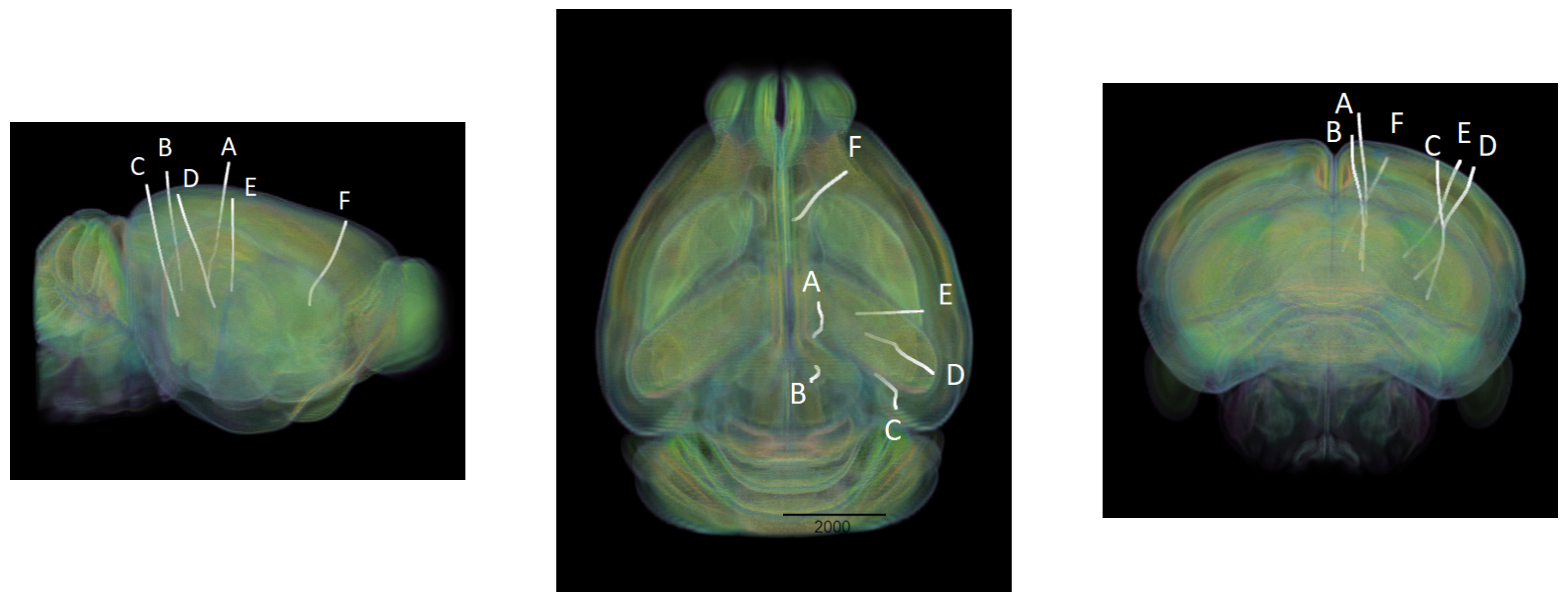
Showing Probe Tracks#
The images below were rendered using the Visualizing Neuropixel Probe Locations notebook. The probes are using the Common Coordinate Framework (CCF). The experiment uses six probes labeled A-F to target various regions.
sagittal_view = Image.open("../../data/images/vippo_probes_sagittal.png")
dorsal_view = Image.open("../../data/images/vippo_probes_dorsal.png")
transverse_view = Image.open("../../data/images/vippo_probes_transverse.png")
fig, axes = plt.subplots(1,3,figsize=(20,60))

axes[0].imshow(sagittal_view)
axes[1].imshow(dorsal_view)
axes[2].imshow(transverse_view)
for ax in axes:
    ax.axis("off")
Extracting Units Spikes#
Below, the Units table is retrieved from the file. It contains many metrics for every putative neuronal unit, printed below. For the analysis in this notebook, we are only interested in the spike_times attribute. This is an array of timestamps that a spike is measured for each unit. For more information on the various unit metrics, see Visualizing Unit Quality Metrics. From this table, the Units used in this notebook are selected if they have ‘good’ quality rather than ‘noise’, and if they belong in one of the regions of the primary visual cortex.
units = nwb.units
units[:10]
| recovery_slope | l_ratio | d_prime | max_drift | firing_rate | isi_violations | presence_ratio | spread | velocity_above | repolarization_slope | ... | PT_ratio | snr | nn_hit_rate | cumulative_drift | amplitude_cutoff | silhouette_score | local_index | spike_times | spike_amplitudes | waveform_mean | |
|---|---|---|---|---|---|---|---|---|---|---|---|---|---|---|---|---|---|---|---|---|---|
| id | |||||||||||||||||||||
| 12 | -0.140852 | 0.000057 | 6.233920 | 31.97 | 1.992914 | 1.224279 | 0.99 | 50.0 | -0.343384 | 0.576991 | ... | 0.596259 | 2.713103 | 0.995333 | 728.41 | 0.498130 | -1.000000 | 0 | [22.76992282041222, 22.783856106625358, 22.812... | [0.00017990238915862748, 0.0001158438415850443... | [[0.0, 0.3712799999999996, 0.2856749999999997,... |
| 13 | -0.120064 | 0.000212 | 6.380643 | 33.91 | 1.516987 | 0.100634 | 0.99 | 30.0 | -0.343384 | 0.818315 | ... | 0.350053 | 4.435071 | 0.992157 | 452.22 | 0.005924 | 0.187985 | 1 | [22.86008918215036, 22.966555488764637, 35.524... | [0.0002144826054165842, 0.0002642146285980156,... | [[0.0, -0.43894499999999814, -0.71662499999999... |
| 14 | -0.061008 | 0.001185 | 4.884140 | 56.95 | 0.703265 | 2.528098 | 0.99 | 40.0 | 0.206030 | 0.241781 | ... | 0.707848 | 2.236984 | 0.929936 | 658.63 | 0.500000 | 0.151979 | 2 | [22.71692299964932, 22.775156136047297, 33.697... | [0.00019346088549011372, 0.0001325490015848021... | [[0.0, -0.30556500000000075, -0.73787999999999... |
| 15 | -0.149691 | 0.002038 | 5.300020 | 6.65 | 0.047692 | 20.360357 | 0.89 | 30.0 | 0.343384 | 0.620252 | ... | 0.635339 | 2.293410 | 0.370370 | 0.00 | 0.160257 | -1.000000 | 3 | [33.70428584210749, 131.43085534614167, 558.25... | [0.00012903155020274154, 0.0001204155056725696... | [[0.0, 0.14145077720207022, 0.8673963730569932... |
| 16 | -0.060737 | 0.001665 | 3.732261 | 39.00 | 0.766648 | 0.078791 | 0.99 | 30.0 | -4.807370 | 0.416142 | ... | 0.722337 | 2.292777 | 0.961187 | 804.07 | 0.006804 | 0.098607 | 4 | [33.670485956413415, 35.54281295782981, 36.159... | [0.00012879827888614498, 0.0001422417048717127... | [[0.0, -0.3408599999999984, -0.251549999999999... |
| 17 | -0.049657 | 0.000373 | 4.709497 | 29.89 | 1.727398 | 0.046559 | 0.99 | 30.0 | 0.000000 | 0.868783 | ... | 0.260276 | 3.844790 | 0.991696 | 368.11 | 0.004070 | 0.265589 | 5 | [20.942295667827928, 22.715523004383883, 22.71... | [0.00017015089162517638, 0.0001707744923264808... | [[0.0, -1.160835000000001, -0.6550050000000008... |
| 18 | -0.043094 | 0.020139 | 3.875737 | 74.63 | 28.778887 | 0.054798 | 0.99 | 70.0 | -0.206030 | 0.565132 | ... | 0.235380 | 2.835290 | 0.904667 | 374.82 | 0.031949 | 0.235098 | 6 | [21.40562743424573, 22.70858969449792, 22.7189... | [0.00027740872559489914, 0.0001854297104938351... | [[0.0, -0.32175000000000087, -0.57954000000000... |
| 19 | -0.142276 | 0.013372 | 4.586741 | 16.11 | 0.192743 | 0.000000 | 0.23 | 50.0 | 0.343384 | 0.789448 | ... | 0.423055 | 3.698435 | 0.154762 | 39.25 | 0.021344 | -1.000000 | 7 | [614.5419882065542, 1230.2982391486003, 1247.0... | [0.0002817193886807515, 0.00034835102540897326... | [[0.0, -1.4075100000000011, -1.464840000000001... |
| 20 | -0.088705 | 0.024535 | 3.589084 | 83.15 | 3.554133 | 0.021996 | 0.93 | 50.0 | 0.343384 | 0.558968 | ... | 0.687279 | 1.877844 | 0.836000 | 395.03 | 0.005054 | 0.181590 | 8 | [291.4390142235864, 291.4497141874008, 291.688... | [0.00021363707722923971, 0.0001794111687378251... | [[0.0, 0.9748050000000008, 2.442375, 2.3462400... |
| 21 | -0.063367 | 0.026352 | 2.811219 | 81.15 | 2.383342 | 0.244578 | 0.95 | 50.0 | 0.000000 | 0.351896 | ... | 0.433562 | 2.194935 | 0.744318 | 413.43 | 0.378081 | 0.037392 | 9 | [141.24085550358953, 232.9827785800948, 293.68... | [0.00013368688760067714, 0.0001396842146963983... | [[0.0, -0.18564000000000025, 0.109785000000000... |
10 rows × 29 columns
nwb.electrodes[:10]
| location | group | group_name | probe_vertical_position | probe_horizontal_position | probe_id | local_index | valid_data | x | y | z | imp | filtering | |
|---|---|---|---|---|---|---|---|---|---|---|---|---|---|
| id | |||||||||||||
| 0 | PF | probeA abc.EcephysElectrodeGroup at 0x22828407... | probeA | 20 | 43 | 0 | 0 | True | 7466.0 | 3423.0 | 6680.0 | NaN | AP band: 500 Hz high-pass; LFP band: 1000 Hz l... |
| 1 | PF | probeA abc.EcephysElectrodeGroup at 0x22828407... | probeA | 20 | 11 | 0 | 1 | True | 7465.0 | 3414.0 | 6682.0 | NaN | AP band: 500 Hz high-pass; LFP band: 1000 Hz l... |
| 2 | PF | probeA abc.EcephysElectrodeGroup at 0x22828407... | probeA | 40 | 59 | 0 | 2 | True | 7465.0 | 3406.0 | 6685.0 | NaN | AP band: 500 Hz high-pass; LFP band: 1000 Hz l... |
| 3 | PF | probeA abc.EcephysElectrodeGroup at 0x22828407... | probeA | 40 | 27 | 0 | 3 | True | 7464.0 | 3397.0 | 6687.0 | NaN | AP band: 500 Hz high-pass; LFP band: 1000 Hz l... |
| 4 | PF | probeA abc.EcephysElectrodeGroup at 0x22828407... | probeA | 60 | 43 | 0 | 4 | True | 7464.0 | 3388.0 | 6690.0 | NaN | AP band: 500 Hz high-pass; LFP band: 1000 Hz l... |
| 5 | TH | probeA abc.EcephysElectrodeGroup at 0x22828407... | probeA | 60 | 11 | 0 | 5 | True | 7463.0 | 3380.0 | 6693.0 | NaN | AP band: 500 Hz high-pass; LFP band: 1000 Hz l... |
| 6 | TH | probeA abc.EcephysElectrodeGroup at 0x22828407... | probeA | 80 | 59 | 0 | 6 | True | 7462.0 | 3371.0 | 6695.0 | NaN | AP band: 500 Hz high-pass; LFP band: 1000 Hz l... |
| 7 | TH | probeA abc.EcephysElectrodeGroup at 0x22828407... | probeA | 80 | 27 | 0 | 7 | True | 7462.0 | 3362.0 | 6698.0 | NaN | AP band: 500 Hz high-pass; LFP band: 1000 Hz l... |
| 8 | TH | probeA abc.EcephysElectrodeGroup at 0x22828407... | probeA | 100 | 43 | 0 | 8 | True | 7461.0 | 3354.0 | 6700.0 | NaN | AP band: 500 Hz high-pass; LFP band: 1000 Hz l... |
| 9 | TH | probeA abc.EcephysElectrodeGroup at 0x22828407... | probeA | 100 | 11 | 0 | 9 | True | 7461.0 | 3345.0 | 6703.0 | NaN | AP band: 500 Hz high-pass; LFP band: 1000 Hz l... |
# select electrodes
channel_locations = {}
channel_probes = {}
channel_idxs = {}

electrodes = nwb.electrodes
for i in range(len(electrodes)):
    channel_id = electrodes["id"][i]
    location = electrodes["location"][i]
    local_idx = electrodes["local_index"][i]
    probe = electrodes["group_name"][i]
    channel_locations[channel_id] = location
    channel_probes[channel_id] = probe
    channel_idxs[channel_id] = local_idx

# function aligns location information from electrodes table with channel id from the units table
def get_unit_location(row):
    return channel_locations[int(row.peak_channel_id)]

def get_unit_probe(row):
    return channel_probes[int(row.peak_channel_id)]

print(set(get_unit_location(row) for row in units))
print(set(channel_probes.values()))
{'VISa6b', 'RSPagl1', 'CA1', 'VPM', 'RSPagl2/3', 'VISli5', 'VPL', 'RSPagl5', 'RT', 'MOp5', 'MOp2/3', 'VISli4', 'DG-mo', 'SSp-bfd2/3', 'VISli6b', 'LP', 'VISa6a', 'TH', 'MOp6b', 'root', 'CP', 'VISli6a', 'PF', 'SSp-bfd6a', 'DG-sg', 'RSPagl6a', 'SSp-bfd4', 'DG-po', 'HPF', 'SSp-bfd5', 'SUB', 'VISli1', 'MOp6a', 'VISli2/3'}
{'probeB', 'probeA', 'probeF', 'probeE'}
### selecting units spike times

brain_regions = ["VISli2/3", "VISa6a", "VISli1", "VISli5", "VISa6b", "VISli6a", "VISli6b", "VISli4"]

# select units based if they have 'good' quality and exists in one of the specified brain_regions
units_spike_times = []
for row in units:
    # if get_unit_location(row) in brain_regions and row.quality.item() == "good":
    if get_unit_location(row) in brain_regions and row.quality.item() == "good":
        units_spike_times.append(row.spike_times.item())

units_spike_times = np.array(units_spike_times, dtype=object)
print(len(units_spike_times))
311
Session Timeline#
# extract epoch times from stim table where stimulus rows have a different 'block' than following row
# returns list of epochs, where an epoch is of the form (stimulus name, stimulus block, start time, stop time)
def extract_epochs(stim_name, stim_table, epochs):

    # specify a current epoch stop and start time
    epoch_start = stim_table.start_time[0]
    epoch_stop = stim_table.stop_time[0]

    # for each row, try to extend current epoch stop_time
    for i in range(len(stim_table)):
        this_block = stim_table.stimulus_block[i]
        # if end of table, end the current epoch
        if i+1 >= len(stim_table):
            epochs.append((stim_name, this_block, epoch_start, epoch_stop))
            break

        next_block = stim_table.stimulus_block[i+1]
        # if next row is the same stim block, push back epoch_stop time
        if next_block == this_block:
            epoch_stop = stim_table.stop_time[i+1]
        # otherwise, end the current epoch, start new epoch
        else:
            epochs.append((stim_name, this_block, epoch_start, epoch_stop))
            epoch_start = stim_table.start_time[i+1]
            epoch_stop = stim_table.stop_time[i+1]

    return epochs
# extract epochs from all valid stimulus tables
epochs = []
for stim_name in nwb.intervals.keys():
    stim_table = nwb.intervals[stim_name]
    try:
        epochs = extract_epochs(stim_name, stim_table, epochs)
    except:
        continue

# manually add optotagging epoch since the table is stored separately
# opto_stim_table = nwb.processing["optotagging"]["optogenetic_stimulation"]
# opto_epoch = ("optogenetic_stimulation", 1.0, opto_stim_table.start_time[0], opto_stim_table.stop_time[-1])
# epochs.append(opto_epoch)

# epochs take the form (stimulus name, stimulus block, start time, stop time)
print(len(epochs))
epochs.sort(key=lambda x: x[2])
for epoch in epochs:
    print(epoch)
21
('SAC_Wd15_Vel2_Bndry1_Cntst0_loop_presentations', 0.0, 113.10293015389608, 593.538290153896)
('SAC_Wd15_Vel2_Bndry2_Cntst0_loop_presentations', 1.0, 593.538290153896, 877.776270153896)
('SAC_Wd15_Vel2_Bndry3_Cntst0_loop_presentations', 2.0, 877.776270153896, 1250.0879201538962)
('SAC_Wd15_Vel8_Bndry1_Cntst0_loop_presentations', 3.0, 1250.0879201538962, 2210.909000153896)
('SAC_Wd45_Vel2_Bndry1_Cntst0_loop_presentations', 4.0, 2210.909000153896, 2451.110230153896)
('SAC_Wd15_Vel2_Bndry1_Cntst1_loop_presentations', 5.0, 2451.110230153896, 2691.311240153896)
('SAC_Wd15_Vel2_Bndry2_Cntst0_oneway_presentations', 6.0, 2691.311240153896, 2833.430250153896)
('UD_Wd15_Vel2_Bndry1_Cntst0_loop_presentations', 7.0, 2833.430250153896, 3313.832440153896)
('Ring_Wd15_Vel2_Bndry1_Cntst0_loop_presentations', 8.0, 3313.832440153896, 3794.234680153896)
('Disk_Wd15_Vel2_Bndry1_Cntst0_loop_presentations', 9.0, 3794.234680153896, 4034.435770153896)
('curl_Wd15_Vel2_Bndry1_Cntst0_oneway_presentations', 10.0, 4034.435770153896, 4154.536360153897)
('acurl_Wd15_Vel2_Bndry1_Cntst0_oneway_presentations', 11.0, 4154.536360153897, 4274.636890153897)
('GreenSAC_Wd15_Vel2_Bndry1_Cntst0_loop_presentations', 12.0, 4274.636890153897, 4514.837970153896)
('Disco2SAC_Wd15_Vel2_Bndry1_Cntst0_loop_presentations', 13.0, 4514.837970153896, 4995.2401701538965)
('natmovie_CricketsOnARock_540x960Full_584x460Active_presentations', 14.0, 4995.2401701538965, 5235.474590153897)
('natmovie_EagleSwooping1_540x960Full_584x460Active_presentations', 15.0, 5235.474590153897, 5475.675670153896)
('natmovie_EagleSwooping2_540x960Full_584x460Active_presentations', 16.0, 5475.675670153896, 5715.876700153896)
('natmovie_SnakeOnARoad_540x960Full_584x460Active_presentations', 17.0, 5715.876700153896, 5956.0777301538965)
('natmovie_Squirreland3Mice_540x960Full_584x460Active_presentations', 18.0, 5956.0777301538965, 6196.312110153896)
('receptive_field_block_presentations', 19.0, 6196.312110153896, 6676.714190153896)
('receptive_field_block_presentations', 20.0, 6676.714190153896, 7157.149566495826)
time_start = floor(min([epoch[2] for epoch in epochs]))
time_end = ceil(max([epoch[3] for epoch in epochs]))
all_units_spike_times = np.concatenate(units_spike_times).ravel()
print(time_start, time_end)

# make histogram of unit spikes per second over specified timeframe
time_bin_edges = np.linspace(time_start, time_end, (time_end-time_start))
hist, bins = np.histogram(all_units_spike_times, bins=time_bin_edges)
113 7158
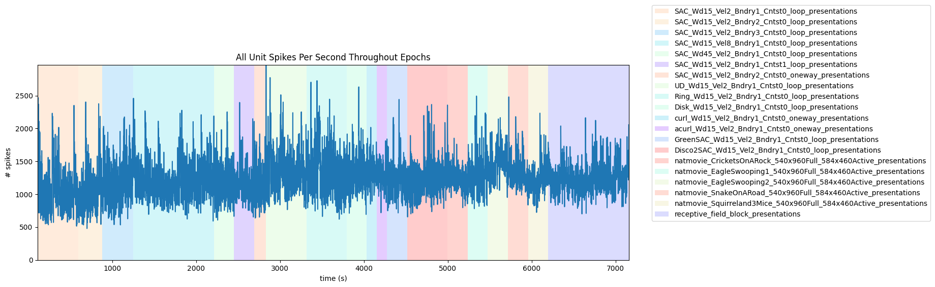
# generate plot of spike histogram with colored epoch intervals and legend
fig, ax = plt.subplots(figsize=(15,5))

# assign unique color to each stimulus name
stim_names = list({epoch[0] for epoch in epochs})
colors = plt.cm.rainbow(np.linspace(0,1,len(stim_names)))
stim_color_map = {stim_names[i]:colors[i] for i in range(len(stim_names))}

epoch_key = {}
height = max(hist)
# draw colored rectangles for each epoch
for epoch in epochs:
    stim_name, stim_block, epoch_start, epoch_end = epoch
    color = stim_color_map[stim_name]
    rec = ax.add_patch(mpl.patches.Rectangle((epoch_start, 0), epoch_end-epoch_start, height, alpha=0.2, facecolor=color))
    epoch_key[stim_name] = rec

ax.set_xlim(time_start, time_end)
ax.set_ylim(-0.1, height+0.1)
ax.set_xlabel("time (s)")
ax.set_ylabel("# spikes")
ax.set_title("All Unit Spikes Per Second Throughout Epochs")

fig.legend(epoch_key.values(), epoch_key.keys(), loc="lower right", bbox_to_anchor=(1.3, 0.25))
ax.plot(bins[:-1], hist)
[<matplotlib.lines.Line2D at 0x213840567d0>]
Extracting Stimulus Times#
nwb.intervals.keys()
dict_keys(['Disco2SAC_Wd15_Vel2_Bndry1_Cntst0_loop_presentations', 'Disk_Wd15_Vel2_Bndry1_Cntst0_loop_presentations', 'GreenSAC_Wd15_Vel2_Bndry1_Cntst0_loop_presentations', 'Ring_Wd15_Vel2_Bndry1_Cntst0_loop_presentations', 'SAC_Wd15_Vel2_Bndry1_Cntst0_loop_presentations', 'SAC_Wd15_Vel2_Bndry1_Cntst1_loop_presentations', 'SAC_Wd15_Vel2_Bndry2_Cntst0_loop_presentations', 'SAC_Wd15_Vel2_Bndry2_Cntst0_oneway_presentations', 'SAC_Wd15_Vel2_Bndry3_Cntst0_loop_presentations', 'SAC_Wd15_Vel8_Bndry1_Cntst0_loop_presentations', 'SAC_Wd45_Vel2_Bndry1_Cntst0_loop_presentations', 'UD_Wd15_Vel2_Bndry1_Cntst0_loop_presentations', 'acurl_Wd15_Vel2_Bndry1_Cntst0_oneway_presentations', 'curl_Wd15_Vel2_Bndry1_Cntst0_oneway_presentations', 'invalid_times', 'natmovie_CricketsOnARock_540x960Full_584x460Active_presentations', 'natmovie_EagleSwooping1_540x960Full_584x460Active_presentations', 'natmovie_EagleSwooping2_540x960Full_584x460Active_presentations', 'natmovie_SnakeOnARoad_540x960Full_584x460Active_presentations', 'natmovie_Squirreland3Mice_540x960Full_584x460Active_presentations', 'receptive_field_block_presentations'])
stim_table = nwb.intervals["SAC_Wd15_Vel2_Bndry1_Cntst0_loop_presentations"]
print(np.mean(np.diff(stim_table.start_time)))
print({elem for elem in stim_table.orientation if not np.isnan(elem)})
0.01668178338976802
{0.0}
stim_table[:10]
| start_time | stop_time | stimulus_name | stimulus_block | frame | color | contrast | opacity | orientation | size | units | stimulus_index | tags | timeseries | |
|---|---|---|---|---|---|---|---|---|---|---|---|---|---|---|
| id | ||||||||||||||
| 0 | 113.102930 | 113.119610 | SAC_Wd15_Vel2_Bndry1_Cntst0_loop | 0.0 | 0.0 | [1.0, 1.0, 1.0] | 1.0 | 1.0 | 0.0 | [1920.0, 1080.0] | pix | 0.0 | [stimulus_time_interval] | [(0, 1, timestamps pynwb.base.TimeSeries at 0x... |
| 1 | 113.119610 | 113.136289 | SAC_Wd15_Vel2_Bndry1_Cntst0_loop | 0.0 | 1.0 | [1.0, 1.0, 1.0] | 1.0 | 1.0 | 0.0 | [1920.0, 1080.0] | pix | 0.0 | [stimulus_time_interval] | [(1, 1, timestamps pynwb.base.TimeSeries at 0x... |
| 2 | 113.136289 | 113.152969 | SAC_Wd15_Vel2_Bndry1_Cntst0_loop | 0.0 | 2.0 | [1.0, 1.0, 1.0] | 1.0 | 1.0 | 0.0 | [1920.0, 1080.0] | pix | 0.0 | [stimulus_time_interval] | [(2, 1, timestamps pynwb.base.TimeSeries at 0x... |
| 3 | 113.152969 | 113.169648 | SAC_Wd15_Vel2_Bndry1_Cntst0_loop | 0.0 | 3.0 | [1.0, 1.0, 1.0] | 1.0 | 1.0 | 0.0 | [1920.0, 1080.0] | pix | 0.0 | [stimulus_time_interval] | [(3, 1, timestamps pynwb.base.TimeSeries at 0x... |
| 4 | 113.169648 | 113.186328 | SAC_Wd15_Vel2_Bndry1_Cntst0_loop | 0.0 | 4.0 | [1.0, 1.0, 1.0] | 1.0 | 1.0 | 0.0 | [1920.0, 1080.0] | pix | 0.0 | [stimulus_time_interval] | [(4, 1, timestamps pynwb.base.TimeSeries at 0x... |
| 5 | 113.186328 | 113.203007 | SAC_Wd15_Vel2_Bndry1_Cntst0_loop | 0.0 | 5.0 | [1.0, 1.0, 1.0] | 1.0 | 1.0 | 0.0 | [1920.0, 1080.0] | pix | 0.0 | [stimulus_time_interval] | [(5, 1, timestamps pynwb.base.TimeSeries at 0x... |
| 6 | 113.203007 | 113.219687 | SAC_Wd15_Vel2_Bndry1_Cntst0_loop | 0.0 | 6.0 | [1.0, 1.0, 1.0] | 1.0 | 1.0 | 0.0 | [1920.0, 1080.0] | pix | 0.0 | [stimulus_time_interval] | [(6, 1, timestamps pynwb.base.TimeSeries at 0x... |
| 7 | 113.219687 | 113.236366 | SAC_Wd15_Vel2_Bndry1_Cntst0_loop | 0.0 | 7.0 | [1.0, 1.0, 1.0] | 1.0 | 1.0 | 0.0 | [1920.0, 1080.0] | pix | 0.0 | [stimulus_time_interval] | [(7, 1, timestamps pynwb.base.TimeSeries at 0x... |
| 8 | 113.236366 | 113.253046 | SAC_Wd15_Vel2_Bndry1_Cntst0_loop | 0.0 | 8.0 | [1.0, 1.0, 1.0] | 1.0 | 1.0 | 0.0 | [1920.0, 1080.0] | pix | 0.0 | [stimulus_time_interval] | [(8, 1, timestamps pynwb.base.TimeSeries at 0x... |
| 9 | 113.253046 | 113.269725 | SAC_Wd15_Vel2_Bndry1_Cntst0_loop | 0.0 | 9.0 | [1.0, 1.0, 1.0] | 1.0 | 1.0 | 0.0 | [1920.0, 1080.0] | pix | 0.0 | [stimulus_time_interval] | [(9, 1, timestamps pynwb.base.TimeSeries at 0x... |
# select times where there is a local oddball
# stim_select = lambda prev_row, row, next_row: prev_row.orientation.item() == 135.0 and row.orientation.item() == 45.0 and np.isnan(next_row.orientation.item())
stim_select = lambda row: float(row.frame) == 40.0
stim_times = [float(stim_table[i].start_time) for i in range(len(stim_table)) if stim_select(stim_table[i])]
print(len(stim_times))
120
Generating Spike Matrix#
# bin size for counting spikes
time_resolution = 0.005

# start and end times (relative to the stimulus at 0 seconds) that we want to examine and align spikes to
window_start_time = -0.25
window_end_time = 0.5
def get_spike_matrix(units_spike_times, stim_times, bin_edges, time_resolution):
    n_units = len(units_spike_times)
    n_trials = len(stim_times)

    # 3D spike matrix to be populated with spike counts
    spike_matrix = np.zeros((n_units, n_trials, len(bin_edges)))

    # populate 3D spike matrix for each unit for each stimulus trial by counting spikes into bins
    for unit_idx in range(n_units):
        spike_times = units_spike_times[unit_idx]

        for stim_idx, stim_time in enumerate(stim_times):
            # get spike times that fall within the bin's time range relative to the stim time
            first_bin_time = stim_time + bin_edges[0]
            last_bin_time = stim_time + bin_edges[-1]
            first_spike_in_range, last_spike_in_range = np.searchsorted(spike_times, [first_bin_time, last_bin_time])
            spike_times_in_range = spike_times[first_spike_in_range:last_spike_in_range]

            # convert spike times into relative time bin indices
            bin_indices = ((spike_times_in_range - (first_bin_time)) / time_resolution).astype(int)

            # mark that there is a spike at these bin times for this unit on this stim trial
            for bin_idx in bin_indices:
                spike_matrix[unit_idx, stim_idx, bin_idx] += 1

    return spike_matrix
# time bins used
n_bins = int((window_end_time - window_start_time) / time_resolution)
bin_edges = np.linspace(window_start_time, window_end_time, n_bins, endpoint=True)

# calculate baseline and stimulus interval indices for use later
stimulus_onset_idx = int(-bin_edges[0] / time_resolution)

spike_matrix = get_spike_matrix(units_spike_times, stim_times, bin_edges, time_resolution)

print(spike_matrix.shape)
(311, 120, 150)
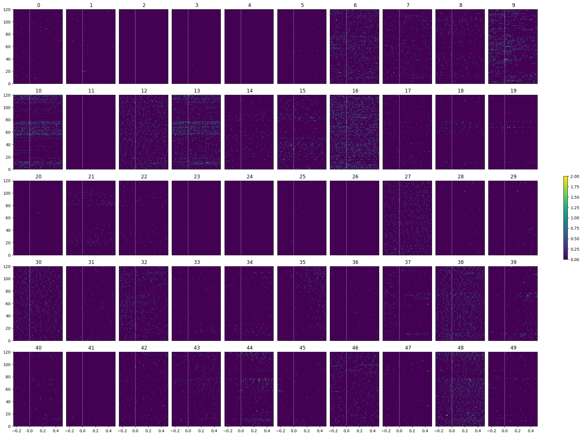
Showing Response Windows#
After generating spike matrices, we can view the PSTHs for each unit.
def show_response(ax, window, window_start_time, window_end_time, aspect="auto", vmin=None, vmax=None, yticklabels=[], skipticks=1, xlabel="Time (s)", ylabel="ROI", cbar=True, cbar_label=None):
    if len(window) == 0:
        print("Input data has length 0; Nothing to display")
        return

    img = ax.imshow(window, aspect=aspect, extent=[window_start_time, window_end_time, 0, len(window)], interpolation="none", vmin=vmin, vmax=vmax)
    if cbar:
        ax.colorbar(img, shrink=0.5, label=cbar_label)

    ax.plot([0,0],[0, len(window)], ":", color="white", linewidth=1.0)

    if len(yticklabels) != 0:
        ax.set_yticks(range(len(yticklabels)))
        ax.set_yticklabels(yticklabels, fontsize=8)

        n_ticks = len(yticklabels[::skipticks])
        ax.yaxis.set_major_locator(plt.MaxNLocator(n_ticks))

    ax.set_xlabel(xlabel)
    ax.set_ylabel(ylabel)
def show_many_responses(windows, rows, cols, window_idxs=None, title=None, subplot_title="", xlabel=None, ylabel=None, cbar_label=None, vmin=0, vmax=2):
    if window_idxs is None:
        window_idxs = range(len(windows))
    windows = windows[window_idxs]

    # handle case with no input data
    if len(windows) == 0:
        print("Input data has length 0; Nothing to display")
        return
    # handle cases when there aren't enough windows for number of rows
    if len(windows) < rows*cols:
        rows = (len(windows) // cols) + 1

    fig, axes = plt.subplots(rows, cols, figsize=(2*cols, 3*rows), layout="constrained")
    # handle case when there's only one row
    if len(axes.shape) == 1:
        axes = axes.reshape((1, axes.shape[0]))

    for i in range(rows*cols):
        ax_row = int(i // cols)
        ax_col = i % cols
        ax = axes[ax_row][ax_col]

        if i > len(windows)-1:
            ax.set_visible(False)
            continue

        window = windows[i]
        show_response(ax, window, window_start_time, window_end_time, xlabel=xlabel, ylabel=ylabel, cbar=False, vmin=vmin, vmax=vmax)
        ax.set_title(f"{subplot_title} {window_idxs[i]}")
        if ax_row != rows-1:
            ax.get_xaxis().set_visible(False)
        if ax_col != 0:
            ax.get_yaxis().set_visible(False)

    fig.suptitle(title)
    norm = mpl.colors.Normalize(vmin=vmin, vmax=vmax)
    colorbar = fig.colorbar(mpl.cm.ScalarMappable(norm=norm), ax=axes, shrink=2/cols, label=cbar_label)
show_many_responses(spike_matrix, 5, 10)
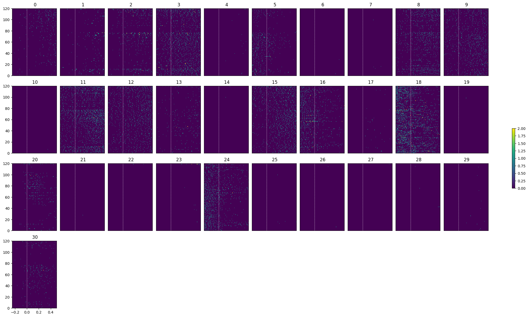
Selecting Responsive Cells#
As discussed in Statistically Testing 2P Responses to Stimulus, the criteria used to select for responsive cells can have a significant impact. Here, the simple criterion is to select units whose post-stimulus z-scores are greater than 1 or less than -1.
def select_cells(spike_matrix, stimulus_onset_idx):
    baseline_means = np.mean(spike_matrix[:,:,:stimulus_onset_idx], axis=2)
    mean_baseline_means = np.mean(baseline_means, axis=1)
    std_baseline_means = np.std(baseline_means, axis=1)

    response_means = np.mean(spike_matrix[:,:,stimulus_onset_idx:], axis=2)
    mean_response_means = np.mean(response_means, axis=1)

    unit_z_scores = (mean_response_means - mean_baseline_means) / std_baseline_means
    return np.where(np.logical_or(unit_z_scores > 1, unit_z_scores < -1))[0]
selected_idxs = select_cells(spike_matrix, stimulus_onset_idx)
show_many_responses(spike_matrix[selected_idxs], 5, 10)
C:\Users\carter.peene\AppData\Local\Temp\ipykernel_30496\1852969462.py:9: RuntimeWarning: divide by zero encountered in divide
  unit_z_scores = (mean_response_means - mean_baseline_means) / std_baseline_means
C:\Users\carter.peene\AppData\Local\Temp\ipykernel_30496\1852969462.py:9: RuntimeWarning: invalid value encountered in divide
  unit_z_scores = (mean_response_means - mean_baseline_means) / std_baseline_means
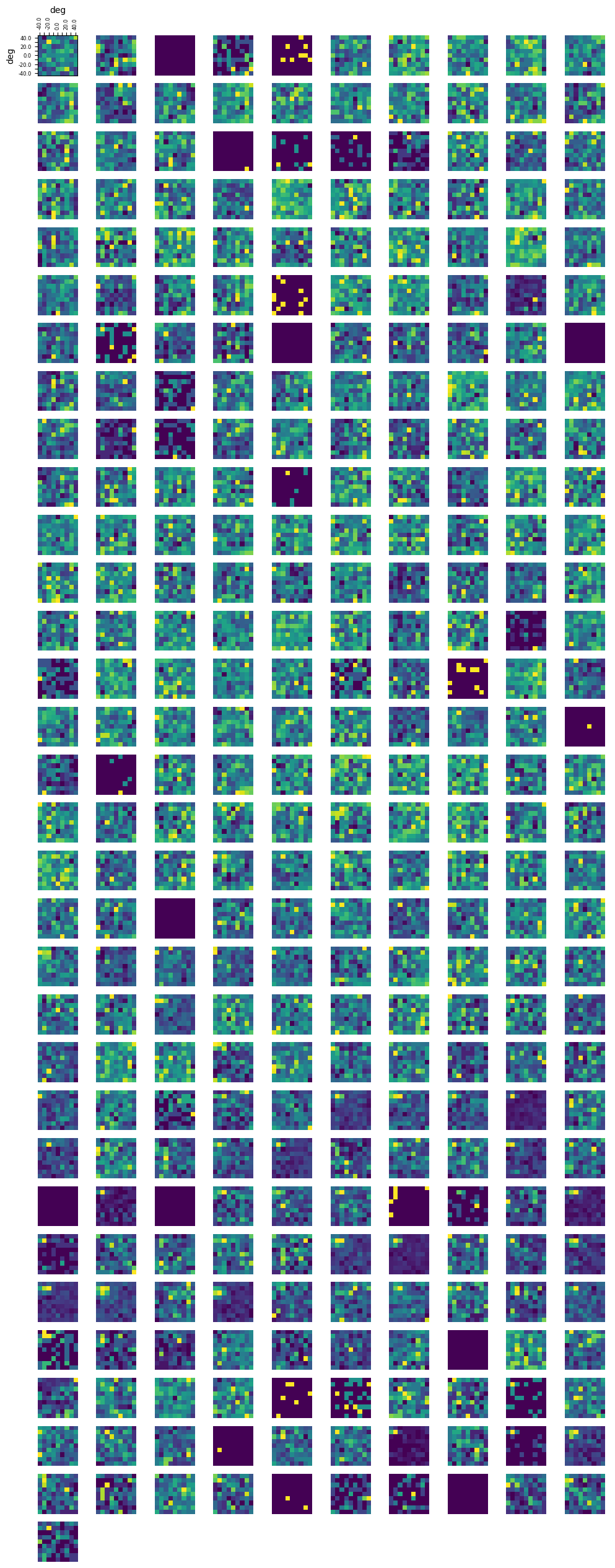
Receptive Fields#
rf_stim_table = nwb.intervals["receptive_field_block_presentations"].to_dataframe()
rf_stim_table[:10]
| start_time | stop_time | stimulus_name | stimulus_block | color | contrast | mask | opacity | orientation | size | units | stimulus_index | temporal_frequency | spatial_frequency | x_position | y_position | phase | tags | timeseries | |
|---|---|---|---|---|---|---|---|---|---|---|---|---|---|---|---|---|---|---|---|
| id | |||||||||||||||||||
| 0 | 6196.312110 | 6196.562318 | receptive_field_block | 19.0 | [1.0, 1.0, 1.0] | 0.8 | circle | 1.0 | 0.0 | [20.0, 20.0] | deg | 19.0 | 4.0 | 0.08 | -10.0 | -30.0 | [26231.93333333, 26231.93333333] | [stimulus_time_interval] | [(364680, 1, timestamps pynwb.base.TimeSeries ... |
| 1 | 6196.562318 | 6196.812525 | receptive_field_block | 19.0 | [1.0, 1.0, 1.0] | 0.8 | circle | 1.0 | 0.0 | [20.0, 20.0] | deg | 19.0 | 4.0 | 0.08 | 20.0 | -30.0 | [26231.93333333, 26231.93333333] | [stimulus_time_interval] | [(364681, 1, timestamps pynwb.base.TimeSeries ... |
| 2 | 6196.812525 | 6197.062733 | receptive_field_block | 19.0 | [1.0, 1.0, 1.0] | 0.8 | circle | 1.0 | 45.0 | [20.0, 20.0] | deg | 19.0 | 4.0 | 0.08 | -10.0 | -30.0 | [26231.93333333, 26231.93333333] | [stimulus_time_interval] | [(364682, 1, timestamps pynwb.base.TimeSeries ... |
| 3 | 6197.062733 | 6197.312941 | receptive_field_block | 19.0 | [1.0, 1.0, 1.0] | 0.8 | circle | 1.0 | 0.0 | [20.0, 20.0] | deg | 19.0 | 4.0 | 0.08 | 30.0 | 10.0 | [26231.93333333, 26231.93333333] | [stimulus_time_interval] | [(364683, 1, timestamps pynwb.base.TimeSeries ... |
| 4 | 6197.312941 | 6197.563156 | receptive_field_block | 19.0 | [1.0, 1.0, 1.0] | 0.8 | circle | 1.0 | 45.0 | [20.0, 20.0] | deg | 19.0 | 4.0 | 0.08 | 20.0 | 40.0 | [26231.93333333, 26231.93333333] | [stimulus_time_interval] | [(364684, 1, timestamps pynwb.base.TimeSeries ... |
| 5 | 6197.563156 | 6197.813370 | receptive_field_block | 19.0 | [1.0, 1.0, 1.0] | 0.8 | circle | 1.0 | 0.0 | [20.0, 20.0] | deg | 19.0 | 4.0 | 0.08 | -40.0 | 10.0 | [26231.93333333, 26231.93333333] | [stimulus_time_interval] | [(364685, 1, timestamps pynwb.base.TimeSeries ... |
| 6 | 6197.813370 | 6198.063585 | receptive_field_block | 19.0 | [1.0, 1.0, 1.0] | 0.8 | circle | 1.0 | 90.0 | [20.0, 20.0] | deg | 19.0 | 4.0 | 0.08 | 20.0 | 30.0 | [26231.93333333, 26231.93333333] | [stimulus_time_interval] | [(364686, 1, timestamps pynwb.base.TimeSeries ... |
| 7 | 6198.063585 | 6198.313800 | receptive_field_block | 19.0 | [1.0, 1.0, 1.0] | 0.8 | circle | 1.0 | 0.0 | [20.0, 20.0] | deg | 19.0 | 4.0 | 0.08 | 20.0 | 40.0 | [26231.93333333, 26231.93333333] | [stimulus_time_interval] | [(364687, 1, timestamps pynwb.base.TimeSeries ... |
| 8 | 6198.313800 | 6198.564005 | receptive_field_block | 19.0 | [1.0, 1.0, 1.0] | 0.8 | circle | 1.0 | 45.0 | [20.0, 20.0] | deg | 19.0 | 4.0 | 0.08 | -40.0 | -30.0 | [26231.93333333, 26231.93333333] | [stimulus_time_interval] | [(364688, 1, timestamps pynwb.base.TimeSeries ... |
| 9 | 6198.564005 | 6198.814210 | receptive_field_block | 19.0 | [1.0, 1.0, 1.0] | 0.8 | circle | 1.0 | 0.0 | [20.0, 20.0] | deg | 19.0 | 4.0 | 0.08 | 0.0 | -40.0 | [26231.93333333, 26231.93333333] | [stimulus_time_interval] | [(364689, 1, timestamps pynwb.base.TimeSeries ... |
### get x and y coordinates of gabors displayed to build receptive field

xs = np.sort(list(set(rf_stim_table.x_position)))
ys = np.sort(list(set(rf_stim_table.y_position)))
field_units = rf_stim_table.units[0]
print(xs)
print(ys)
print(field_units)
[-40. -30. -20. -10.   0.  10.  20.  30.  40.]
[-40. -30. -20. -10.   0.  10.  20.  30.  40.]
deg
### get receptive field of a unit using its spike times and the stim table

def get_rf(spike_times):
    # creates 2D array that stores response spike counts for each coordinate of the receptive field
    unit_rf = np.zeros([ys.size, xs.size])
    # for every x and y coordinate in the field
    for xi, x in enumerate(xs):
        for yi, y in enumerate(ys):

            # for this coordinate of the rf, count all the times that this neuron responds to a stimulus time with a spike
            stim_times = rf_stim_table[(rf_stim_table.x_position == x) & (rf_stim_table.y_position == y)].start_time
            response_spike_count = 0
            for stim_time in stim_times:
                # any spike within 0.2 seconds after stim time is considered a response
                start_idx, end_idx = np.searchsorted(spike_times, [stim_time, stim_time+0.2])
                response_spike_count += end_idx-start_idx

            unit_rf[yi, xi] = response_spike_count

    return unit_rf
### compute receptive fields for each unit in selected units

rfs = []
# for idx in selected_idxs:
for idx in range(spike_matrix.shape[0]):
    these_spike_times = units_spike_times[idx]
    rfs.append(get_rf(these_spike_times))
### display the receptive fields for each unit in a 2D plot

def display_rfs(rfs, n_cols=10):
    if len(rfs) == 0:
        print("No receptive fields provided. Nothing to display")
        return

    n_rows = len(rfs) // n_cols
    fig, axes = plt.subplots(n_rows+1, 10)
    fig.set_size_inches(12, n_rows+1)

    # handle case where there's <= n_cols rfs
    if len(axes.shape) == 1:
        axes = axes.reshape((1, axes.shape[0]))

    for irf, rf in enumerate(rfs):
        ax_row = int(irf/10)
        ax_col = irf%10
        axes[ax_row][ax_col].imshow(rf, origin="lower")
    for ax in axes.flat[1:]:
        ax.axis('off')

    # making axis labels for first receptive field
    axes[0][0].set_xlabel(field_units)
    axes[0][0].set_ylabel(field_units)
    axes[0][0].xaxis.set_label_position("top")
    axes[0][0].xaxis.set_ticks_position("top")
    axes[0][0].set_xticks(range(len(xs)), xs, rotation=90, fontsize=6)
    axes[0][0].set_yticks(range(len(ys)), ys, fontsize=6)
    [l.set_visible(False) for (i,l) in enumerate(axes[0][0].xaxis.get_ticklabels()) if i % 2 != 0]
    [l.set_visible(False) for (i,l) in enumerate(axes[0][0].yaxis.get_ticklabels()) if i % 2 != 0]
display_rfs(rfs)