Generalized Linear Models#
A Generalized Linear Model (GLM), not to be confused with a General Linear Model, is a regression model that trains a filter to model single neuron activity as it relates to some other variable. For example, to predict the spike counts produced by a single neuron (Y) in response to licking events (X). The GLM model can be represented by the following equation:
\(y(t) = Poiss(f(k * X_{t}))\), where Poiss is a poisson process and f is a non-linearity function, in this case \(f(x) = e^x\)
To train a GLM, we start by creating a design matrix from the visual stimulus. The design matrix is the input, X_train, provided to the GLM for training along with known spike counts in each trial, Y_train. The GLM uses Maximum Likelihood Estimation to train the filter vector that maximizes the likelihood of producing a given spike train from the inputted design matrix. To predict the spike activity of a neuron, the filter is first convolved with the stimulus vector. Next, the GLM employs a non-linearity step (exponential in this case), followed by poisson generation to generate specific spike counts as shown in the figure below.
This notebook demonstrates the usage of a Poisson GLM to model and reproduce the spiking activity of single neurons in response to a visual stimulus. GLMs are trained using synthetic data, as well as real data from the Allen Institute Visual Coding - Neuropixels dataset.
For more information on applying GLMs for predicting spiking activity, see the Pillow Lab’s GLM Slides and Neuromatch Academy’s GLM tutorial.
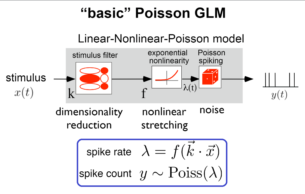
Modified from Slide 6, Generalized linear models for cracking the neural code, Pillow Lab
Environment Setup#
try:
    from databook_utils.dandi_utils import dandi_download_open
except:
    !git clone https://github.com/AllenInstitute/openscope_databook.git
    %cd openscope_databook
    %pip install -e .
import os
import numpy as np

import matplotlib.pyplot as plt
import statsmodels.api as sm

from math import ceil
from scipy import interpolate
from functools import reduce

from scipy.optimize import minimize
from sklearn.metrics import r2_score

%matplotlib inline
Downloading File#
dandiset_id = "000021"
dandi_filepath = "sub-726298249/sub-726298249_ses-754829445.nwb"
download_loc = "."
io = dandi_download_open(dandiset_id, dandi_filepath, download_loc)
nwb = io.read()
A newer version (0.62.2) of dandi/dandi-cli is available. You are using 0.61.2
File already exists
Opening file
c:\Users\carter.peene\Desktop\Projects\openscope_databook\databook_env\lib\site-packages\hdmf\utils.py:668: UserWarning: Ignoring cached namespace 'hdmf-common' version 1.1.3 because version 1.8.0 is already loaded.
  return func(args[0], **pargs)
c:\Users\carter.peene\Desktop\Projects\openscope_databook\databook_env\lib\site-packages\hdmf\utils.py:668: UserWarning: Ignoring cached namespace 'core' version 2.2.2 because version 2.6.0-alpha is already loaded.
  return func(args[0], **pargs)
The GLM#
The functions below are used in training the GLM.
The function fit_lnp takes in the design_matrix ~as~, X, produced from the stimulus and the observed spike counts, y. It also takes the length of the filter to train, d, and the regularization coefficient, lam,. First, the function initializes a random filter of length d and then uses the neg_log_like_lnp function to perform Maximum Likelihood Estimation to train the filter.
neg_log_lik_lnp computes the negative log likelihood for a vector of filter weights theta, the design matrix X, and the observed spike counts, y. The Cinv matrix, a diagonal matrix with the regularization coefficient, is applied for regularization. It would also help to explain each function by its inputs and outputs.
The predict function perform the inverse operation, applying a trained filter weights to the design matrix X, and adding a constant, yielding the spike probability over time.
predict_spikes takes the spike rate prediction and runs it through Poisson generation, adding noise and producing a set of predicted spike counts. Because the poisson generation is non-deterministic, it will produce different results every time.
This code was adapted from this code from the Pillow Lab, with the regularization code from this tutorial from Neuromatch Academy.
def neg_log_lik_lnp(theta, X, y, Cinv):
  # Compute the Poisson log likelihood
  rate = np.exp(X @ theta)
  log_lik = y @ np.log(rate) - rate.sum()
  log_lik -= theta.T @ Cinv @ theta

  return -log_lik
def fit_lnp(X, y, lam=0):
  filt_len = X.shape[1]
  Imat = np.identity(filt_len) # identity matrix of size of filter + const
  Imat[0,0] = 0
  Cinv = lam*Imat

  # Use a random vector of weights to start (mean 0, sd .2)
  x0 = np.random.normal(0, .2, filt_len)
  print("y:",y.shape,"X:",X.shape,"x0:",x0.shape)

  # Find parameters that minimize the negative log likelihood function
  res = minimize(neg_log_lik_lnp, x0, args=(X, y, Cinv))

  return res["x"]
def predict(X, weights, constant):
    y = np.exp(X @ weights + constant)
    return y

def predict_spikes(X, weights, constant):
    rate = predict(X, weights, constant)
    spks = np.random.poisson(np.matrix.transpose(rate))
    return spks
Synthetic Data#
The cells below prepare the synthetic data (stimulus and spiking data), and show how to train a GLM.
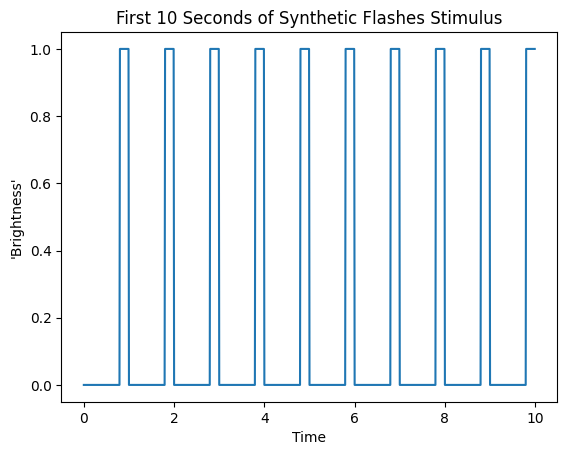
make_flashes produces boxcar stimulus that imitate binary flashes.
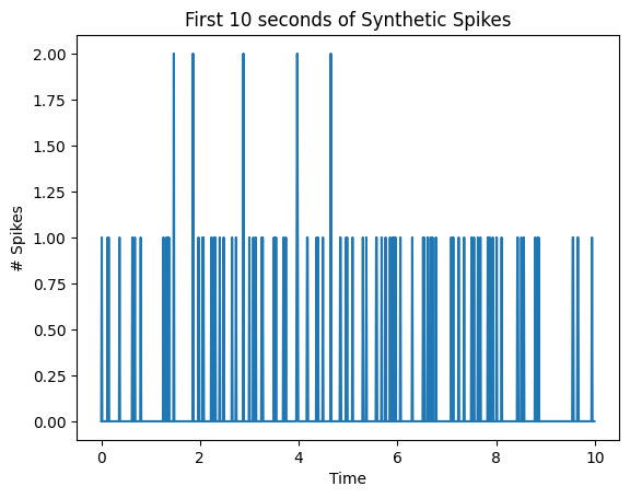
make_spikes utilizes the same mathematics as the GLM’s prediction and generates spikes that have a direct relationship with the brightness of the synthetic stimulus. It simply multiplies the stimulus by a given coefficient coeff, and adds a given constant, baseline_rate. It runs the resulting rate through exponentiation and then generates Poission distributed spike counts with this as the spiking probability.
def make_flashes(time_start, time_end, pattern, n_repeats):
    flashes = np.tile(pattern, n_repeats)
    time_axis = np.linspace(time_start, time_end, len(flashes))
    return time_axis, flashes

syn_time_axis, syn_flashes = make_flashes(0, 300, [0]*80 + [1]*20, 300)
print(syn_time_axis[0], syn_time_axis[-1])
print(len(syn_flashes))

plt.plot(syn_time_axis[:1000], syn_flashes[:1000])
plt.title("First 10 Seconds of Synthetic Flashes Stimulus")
plt.xlabel("Time")
plt.ylabel("'Brightness'")
0.0 300.0
30000
Text(0, 0.5, "'Brightness'")
def make_spikes(stim, baseline_rate, coeff, return_exp=False):
    weighted_stim = (stim*coeff) + baseline_rate
    exp_stim = np.exp(weighted_stim)
    print(np.max(exp_stim), np.min(exp_stim))
    spikes = np.random.poisson(exp_stim)
    if return_exp:
        return spikes, weighted_stim, exp_stim
    return spikes

# set with parameters -2.5 and 0.5, the GLM should learn these parameters
syn_spikes, syn_weight, syn_exp = make_spikes(syn_flashes, -2.5, 0.5, return_exp=True)
print(len(syn_spikes))

plt.plot(syn_time_axis[:1000], syn_spikes[:1000])
plt.title("First 10 seconds of Synthetic Spikes")
plt.xlabel("Time")
plt.ylabel("# Spikes")
0.1353352832366127 0.0820849986238988
30000
Text(0, 0.5, '# Spikes')
Design Matrix#
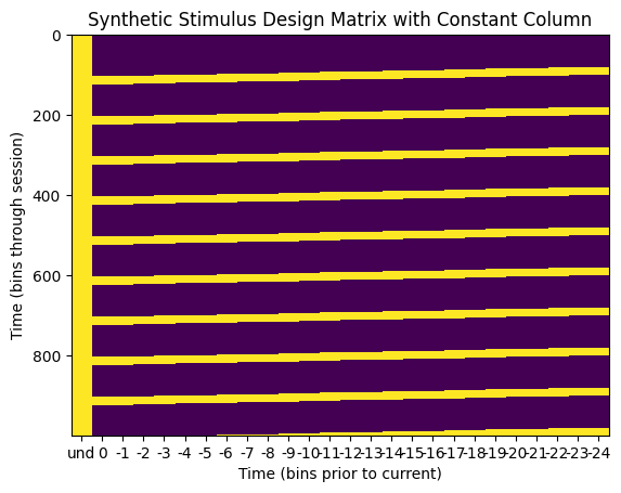
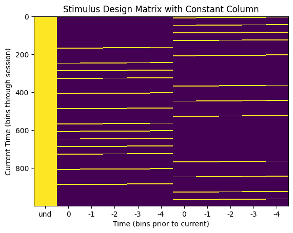
The GLM takes in the following design matrix to conduct Maximum Likelihood Estimation. The design matrix must have dimensions time * d, where time is the length of the stimulus, and d is the length of the filter to be trained. It can be seen below that it is simply slices of the d most recent stimulus values for each timepoint in the stimulus. Importantly, a GLM also yields a constant value with each filter. This constant term is the bias term that captures the spike count variance unexplained by the input variables. For this, we simply add a 1 to each row in the design matrix. The resulting column of 1s produces the bias term from the MLE.
The function build_design_matrix returns such a design_matrix from a given stim array and a filter length d. It can be seen below that the bins of the second dimension of the design matrix represent the stimulus values preceding the stimulus event, so the time axis is time prior the ‘current time’. The column of ones to product the GLM constant does not have a temporal relationship to the latest stimulus time, so its x value in the matrix undefined.
def build_design_mat(stim, d, include_const=True):
  # Create version of stimulus vector with zeros before onset
  padded_stim = np.concatenate([np.zeros(d-1), stim])

  # Construct a matrix where each row has the d frames of
  # the stimulus preceding and including timepoint t
  T = len(stim)  # Total number of timepoints (hint: number of stimulus frames)
  X = np.zeros((T, d))
  for t in range(T):
      X[t] = padded_stim[t:t + d]

  if include_const:
    constant = np.ones_like(stim)
    return np.column_stack([constant, X])
  return X
syn_design_mat = build_design_mat(syn_flashes, 25)
print(syn_design_mat.shape)
plt.imshow(syn_design_mat[:1000], aspect="auto", interpolation="none")
plt.xlabel("Time (bins prior to current)")
xaxis_step = 1
xpositions = range(0,syn_design_mat.shape[1])[::xaxis_step]
time_offset_axis = range(0,-syn_design_mat.shape[1]+1,-1)
xticks = (["und"] + list(time_offset_axis))[::xaxis_step]
plt.xticks(xpositions, xticks)
plt.ylabel("Time (bins through session)")
plt.title("Synthetic Stimulus Design Matrix with Constant Column")
(30000, 26)
Text(0.5, 1.0, 'Synthetic Stimulus Design Matrix with Constant Column')
Running on Synthetic Data#
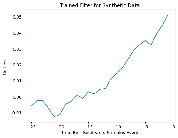
Below is an example of a trained GLM filter trained using a filter length of 25 and a regularization coefficient of \(2^{10}\). During prediction, this filter would be convolved with the design matrix before undergoing the exponential non-linearity step to produce spike rate.
res = fit_lnp(syn_design_mat, syn_spikes, lam=2**10)
constant, filter = res[0], res[1:]
print(constant)
plt.plot(range(-len(filter),0), filter)
plt.title("Trained Filter for Synthetic Data")
plt.xlabel("Time Bins Relative to Stimulus Event")
plt.ylabel("Unitless")
y: (30000,) X: (30000, 26) x0: (26,)
-2.4325110136550547
Text(0, 0.5, 'Unitless')
Testing Model#
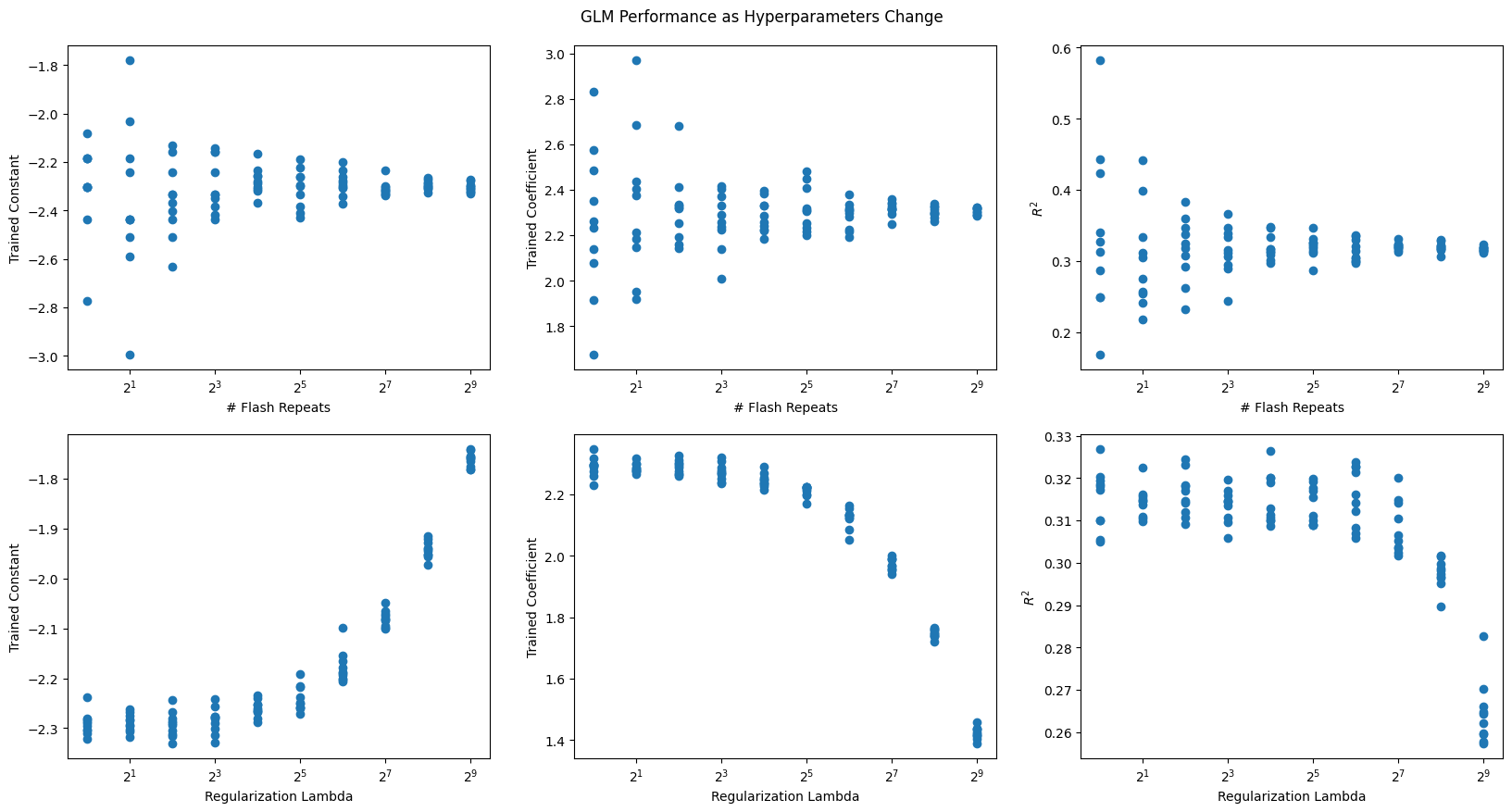
To get a sense of how the GLM performs on synthetic data, the function test_synthetic_glm is used to yield a constant and a filter of length 1. Since the synthetic spikes were produced with a constant baseline_rate and a coefficient coeff, we should expect the GLM to effectively reproduce these values in the constant and length 1 filter. The GLM performance is tested by iterating over successive values of regularization coefficient lam and the number of repeats of stimulus flashes, n_repeats, both ranging between 1 and \(2^9\). The optimal values for these variables are obtained by maximixing the Coefficient of Determination \(R^2\). The results below indicate that as the regularization coefficient increases, the GLM performance starts to suffer. This is because higher regularization values promote a stronger tendency for trained filter values to stay closer to 0, limiting the MLE’s ability to fit a model effectively. They also indicate that the GLM performance converges toward the real constant and coefficient values as the number of repeats of the stimulus increases because there is more data to train with.
def test_synthetic_glm(constant_in, coeff_in, flashes, constants, filters, r2s, lam=0, filt_len=1):
    design_mat = build_design_mat(flashes, d=filt_len)
    syn_spikes, syn_weights, syn_prob = make_spikes(flashes, constant_in, coeff_in, return_exp=True)

    res = fit_lnp(design_mat, syn_spikes, lam=lam)
    const, filt = res[0], res[1:]

    prob_predicted = predict(design_mat[:,1:], filt, const)
    spikes_predicted = predict_spikes(design_mat[:,1:], filt, const)
    r2 = r2_score(syn_spikes, prob_predicted)

    constants.append(const)
    filters.append(filt)
    r2s.append(r2)
repeats_vals = []
r_coeffs = []
r_constants = []
r_r2s = []

for i in range(10):
    n_repeats = 2**i
    time_axis, syn_flashes = make_flashes(0, n_repeats, [0]*80 + [1]*20, n_repeats)

    for j in range(10):
        test_synthetic_glm(-2.3, 2.3, syn_flashes, r_constants, r_coeffs, r_r2s)
        repeats_vals.append(n_repeats)

lambda_vals = []
l_coeffs = []
l_constants = []
l_r2s = []

time_axis, syn_flashes = make_flashes(0, 2**8, [0]*80 + [1]*20, 2**8)
design_mat = build_design_mat(syn_flashes, d=2)
for i in range(10):
    lam = 2**i

    for j in range(10):
        test_synthetic_glm(-2.3, 2.3, syn_flashes, l_constants, l_coeffs, l_r2s, lam=lam)
        lambda_vals.append(lam)
1.0 0.10025884372280375
y: (100,) X: (100, 2) x0: (2,)
1.0 0.10025884372280375
y: (100,) X: (100, 2) x0: (2,)
1.0 0.10025884372280375
y: (100,) X: (100, 2) x0: (2,)
1.0 0.10025884372280375
y: (100,) X: (100, 2) x0: (2,)
1.0 0.10025884372280375
y: (100,) X: (100, 2) x0: (2,)
1.0 0.10025884372280375
y: (100,) X: (100, 2) x0: (2,)
1.0 0.10025884372280375
y: (100,) X: (100, 2) x0: (2,)
1.0 0.10025884372280375
y: (100,) X: (100, 2) x0: (2,)
1.0 0.10025884372280375
y: (100,) X: (100, 2) x0: (2,)
1.0 0.10025884372280375
y: (100,) X: (100, 2) x0: (2,)
1.0 0.10025884372280375
y: (200,) X: (200, 2) x0: (2,)
1.0 0.10025884372280375
y: (200,) X: (200, 2) x0: (2,)
1.0 0.10025884372280375
y: (200,) X: (200, 2) x0: (2,)
1.0 0.10025884372280375
y: (200,) X: (200, 2) x0: (2,)
1.0 0.10025884372280375
y: (200,) X: (200, 2) x0: (2,)
1.0 0.10025884372280375
y: (200,) X: (200, 2) x0: (2,)
1.0 0.10025884372280375
y: (200,) X: (200, 2) x0: (2,)
1.0 0.10025884372280375
y: (200,) X: (200, 2) x0: (2,)
1.0 0.10025884372280375
y: (200,) X: (200, 2) x0: (2,)
1.0 0.10025884372280375
y: (200,) X: (200, 2) x0: (2,)
1.0 0.10025884372280375
y: (400,) X: (400, 2) x0: (2,)
1.0 0.10025884372280375
y: (400,) X: (400, 2) x0: (2,)
1.0 0.10025884372280375
y: (400,) X: (400, 2) x0: (2,)
1.0 0.10025884372280375
y: (400,) X: (400, 2) x0: (2,)
1.0 0.10025884372280375
y: (400,) X: (400, 2) x0: (2,)
1.0 0.10025884372280375
y: (400,) X: (400, 2) x0: (2,)
1.0 0.10025884372280375
y: (400,) X: (400, 2) x0: (2,)
1.0 0.10025884372280375
y: (400,) X: (400, 2) x0: (2,)
1.0 0.10025884372280375
y: (400,) X: (400, 2) x0: (2,)
1.0 0.10025884372280375
y: (400,) X: (400, 2) x0: (2,)
1.0 0.10025884372280375
y: (800,) X: (800, 2) x0: (2,)
1.0 0.10025884372280375
y: (800,) X: (800, 2) x0: (2,)
1.0 0.10025884372280375
y: (800,) X: (800, 2) x0: (2,)
1.0 0.10025884372280375
y: (800,) X: (800, 2) x0: (2,)
1.0 0.10025884372280375
y: (800,) X: (800, 2) x0: (2,)
1.0 0.10025884372280375
y: (800,) X: (800, 2) x0: (2,)
1.0 0.10025884372280375
y: (800,) X: (800, 2) x0: (2,)
1.0 0.10025884372280375
y: (800,) X: (800, 2) x0: (2,)
1.0 0.10025884372280375
y: (800,) X: (800, 2) x0: (2,)
1.0 0.10025884372280375
y: (800,) X: (800, 2) x0: (2,)
1.0 0.10025884372280375
y: (1600,) X: (1600, 2) x0: (2,)
1.0 0.10025884372280375
y: (1600,) X: (1600, 2) x0: (2,)
1.0 0.10025884372280375
y: (1600,) X: (1600, 2) x0: (2,)
1.0 0.10025884372280375
y: (1600,) X: (1600, 2) x0: (2,)
1.0 0.10025884372280375
y: (1600,) X: (1600, 2) x0: (2,)
1.0 0.10025884372280375
y: (1600,) X: (1600, 2) x0: (2,)
1.0 0.10025884372280375
y: (1600,) X: (1600, 2) x0: (2,)
1.0 0.10025884372280375
y: (1600,) X: (1600, 2) x0: (2,)
1.0 0.10025884372280375
y: (1600,) X: (1600, 2) x0: (2,)
1.0 0.10025884372280375
y: (1600,) X: (1600, 2) x0: (2,)
1.0 0.10025884372280375
y: (3200,) X: (3200, 2) x0: (2,)
1.0 0.10025884372280375
y: (3200,) X: (3200, 2) x0: (2,)
1.0 0.10025884372280375
y: (3200,) X: (3200, 2) x0: (2,)
1.0 0.10025884372280375
y: (3200,) X: (3200, 2) x0: (2,)
1.0 0.10025884372280375
y: (3200,) X: (3200, 2) x0: (2,)
1.0 0.10025884372280375
y: (3200,) X: (3200, 2) x0: (2,)
1.0 0.10025884372280375
y: (3200,) X: (3200, 2) x0: (2,)
1.0 0.10025884372280375
y: (3200,) X: (3200, 2) x0: (2,)
1.0 0.10025884372280375
y: (3200,) X: (3200, 2) x0: (2,)
1.0 0.10025884372280375
y: (3200,) X: (3200, 2) x0: (2,)
1.0 0.10025884372280375
y: (6400,) X: (6400, 2) x0: (2,)
1.0 0.10025884372280375
y: (6400,) X: (6400, 2) x0: (2,)
1.0 0.10025884372280375
y: (6400,) X: (6400, 2) x0: (2,)
1.0 0.10025884372280375
y: (6400,) X: (6400, 2) x0: (2,)
1.0 0.10025884372280375
y: (6400,) X: (6400, 2) x0: (2,)
1.0 0.10025884372280375
y: (6400,) X: (6400, 2) x0: (2,)
1.0 0.10025884372280375
y: (6400,) X: (6400, 2) x0: (2,)
1.0 0.10025884372280375
y: (6400,) X: (6400, 2) x0: (2,)
1.0 0.10025884372280375
y: (6400,) X: (6400, 2) x0: (2,)
1.0 0.10025884372280375
y: (6400,) X: (6400, 2) x0: (2,)
1.0 0.10025884372280375
y: (12800,) X: (12800, 2) x0: (2,)
1.0 0.10025884372280375
y: (12800,) X: (12800, 2) x0: (2,)
1.0 0.10025884372280375
y: (12800,) X: (12800, 2) x0: (2,)
1.0 0.10025884372280375
y: (12800,) X: (12800, 2) x0: (2,)
1.0 0.10025884372280375
y: (12800,) X: (12800, 2) x0: (2,)
1.0 0.10025884372280375
y: (12800,) X: (12800, 2) x0: (2,)
1.0 0.10025884372280375
y: (12800,) X: (12800, 2) x0: (2,)
1.0 0.10025884372280375
y: (12800,) X: (12800, 2) x0: (2,)
1.0 0.10025884372280375
y: (12800,) X: (12800, 2) x0: (2,)
1.0 0.10025884372280375
y: (12800,) X: (12800, 2) x0: (2,)
1.0 0.10025884372280375
y: (25600,) X: (25600, 2) x0: (2,)
1.0 0.10025884372280375
y: (25600,) X: (25600, 2) x0: (2,)
1.0 0.10025884372280375
y: (25600,) X: (25600, 2) x0: (2,)
1.0 0.10025884372280375
y: (25600,) X: (25600, 2) x0: (2,)
1.0 0.10025884372280375
y: (25600,) X: (25600, 2) x0: (2,)
1.0 0.10025884372280375
y: (25600,) X: (25600, 2) x0: (2,)
1.0 0.10025884372280375
y: (25600,) X: (25600, 2) x0: (2,)
1.0 0.10025884372280375
y: (25600,) X: (25600, 2) x0: (2,)
1.0 0.10025884372280375
y: (25600,) X: (25600, 2) x0: (2,)
1.0 0.10025884372280375
y: (25600,) X: (25600, 2) x0: (2,)
1.0 0.10025884372280375
y: (51200,) X: (51200, 2) x0: (2,)
1.0 0.10025884372280375
y: (51200,) X: (51200, 2) x0: (2,)
1.0 0.10025884372280375
y: (51200,) X: (51200, 2) x0: (2,)
1.0 0.10025884372280375
y: (51200,) X: (51200, 2) x0: (2,)
1.0 0.10025884372280375
y: (51200,) X: (51200, 2) x0: (2,)
1.0 0.10025884372280375
y: (51200,) X: (51200, 2) x0: (2,)
1.0 0.10025884372280375
y: (51200,) X: (51200, 2) x0: (2,)
1.0 0.10025884372280375
y: (51200,) X: (51200, 2) x0: (2,)
1.0 0.10025884372280375
y: (51200,) X: (51200, 2) x0: (2,)
1.0 0.10025884372280375
y: (51200,) X: (51200, 2) x0: (2,)
1.0 0.10025884372280375
y: (25600,) X: (25600, 2) x0: (2,)
1.0 0.10025884372280375
y: (25600,) X: (25600, 2) x0: (2,)
1.0 0.10025884372280375
y: (25600,) X: (25600, 2) x0: (2,)
1.0 0.10025884372280375
y: (25600,) X: (25600, 2) x0: (2,)
1.0 0.10025884372280375
y: (25600,) X: (25600, 2) x0: (2,)
1.0 0.10025884372280375
y: (25600,) X: (25600, 2) x0: (2,)
1.0 0.10025884372280375
y: (25600,) X: (25600, 2) x0: (2,)
1.0 0.10025884372280375
y: (25600,) X: (25600, 2) x0: (2,)
1.0 0.10025884372280375
y: (25600,) X: (25600, 2) x0: (2,)
1.0 0.10025884372280375
y: (25600,) X: (25600, 2) x0: (2,)
1.0 0.10025884372280375
y: (25600,) X: (25600, 2) x0: (2,)
1.0 0.10025884372280375
y: (25600,) X: (25600, 2) x0: (2,)
1.0 0.10025884372280375
y: (25600,) X: (25600, 2) x0: (2,)
1.0 0.10025884372280375
y: (25600,) X: (25600, 2) x0: (2,)
1.0 0.10025884372280375
y: (25600,) X: (25600, 2) x0: (2,)
1.0 0.10025884372280375
y: (25600,) X: (25600, 2) x0: (2,)
1.0 0.10025884372280375
y: (25600,) X: (25600, 2) x0: (2,)
1.0 0.10025884372280375
y: (25600,) X: (25600, 2) x0: (2,)
1.0 0.10025884372280375
y: (25600,) X: (25600, 2) x0: (2,)
1.0 0.10025884372280375
y: (25600,) X: (25600, 2) x0: (2,)
1.0 0.10025884372280375
y: (25600,) X: (25600, 2) x0: (2,)
1.0 0.10025884372280375
y: (25600,) X: (25600, 2) x0: (2,)
1.0 0.10025884372280375
y: (25600,) X: (25600, 2) x0: (2,)
1.0 0.10025884372280375
y: (25600,) X: (25600, 2) x0: (2,)
1.0 0.10025884372280375
y: (25600,) X: (25600, 2) x0: (2,)
1.0 0.10025884372280375
y: (25600,) X: (25600, 2) x0: (2,)
1.0 0.10025884372280375
y: (25600,) X: (25600, 2) x0: (2,)
1.0 0.10025884372280375
y: (25600,) X: (25600, 2) x0: (2,)
1.0 0.10025884372280375
y: (25600,) X: (25600, 2) x0: (2,)
1.0 0.10025884372280375
y: (25600,) X: (25600, 2) x0: (2,)
1.0 0.10025884372280375
y: (25600,) X: (25600, 2) x0: (2,)
1.0 0.10025884372280375
y: (25600,) X: (25600, 2) x0: (2,)
1.0 0.10025884372280375
y: (25600,) X: (25600, 2) x0: (2,)
1.0 0.10025884372280375
y: (25600,) X: (25600, 2) x0: (2,)
1.0 0.10025884372280375
y: (25600,) X: (25600, 2) x0: (2,)
1.0 0.10025884372280375
y: (25600,) X: (25600, 2) x0: (2,)
1.0 0.10025884372280375
y: (25600,) X: (25600, 2) x0: (2,)
1.0 0.10025884372280375
y: (25600,) X: (25600, 2) x0: (2,)
1.0 0.10025884372280375
y: (25600,) X: (25600, 2) x0: (2,)
1.0 0.10025884372280375
y: (25600,) X: (25600, 2) x0: (2,)
1.0 0.10025884372280375
y: (25600,) X: (25600, 2) x0: (2,)
1.0 0.10025884372280375
y: (25600,) X: (25600, 2) x0: (2,)
1.0 0.10025884372280375
y: (25600,) X: (25600, 2) x0: (2,)
1.0 0.10025884372280375
y: (25600,) X: (25600, 2) x0: (2,)
1.0 0.10025884372280375
y: (25600,) X: (25600, 2) x0: (2,)
1.0 0.10025884372280375
y: (25600,) X: (25600, 2) x0: (2,)
1.0 0.10025884372280375
y: (25600,) X: (25600, 2) x0: (2,)
1.0 0.10025884372280375
y: (25600,) X: (25600, 2) x0: (2,)
1.0 0.10025884372280375
y: (25600,) X: (25600, 2) x0: (2,)
1.0 0.10025884372280375
y: (25600,) X: (25600, 2) x0: (2,)
1.0 0.10025884372280375
y: (25600,) X: (25600, 2) x0: (2,)
1.0 0.10025884372280375
y: (25600,) X: (25600, 2) x0: (2,)
1.0 0.10025884372280375
y: (25600,) X: (25600, 2) x0: (2,)
1.0 0.10025884372280375
y: (25600,) X: (25600, 2) x0: (2,)
1.0 0.10025884372280375
y: (25600,) X: (25600, 2) x0: (2,)
1.0 0.10025884372280375
y: (25600,) X: (25600, 2) x0: (2,)
1.0 0.10025884372280375
y: (25600,) X: (25600, 2) x0: (2,)
1.0 0.10025884372280375
y: (25600,) X: (25600, 2) x0: (2,)
1.0 0.10025884372280375
y: (25600,) X: (25600, 2) x0: (2,)
1.0 0.10025884372280375
y: (25600,) X: (25600, 2) x0: (2,)
1.0 0.10025884372280375
y: (25600,) X: (25600, 2) x0: (2,)
1.0 0.10025884372280375
y: (25600,) X: (25600, 2) x0: (2,)
1.0 0.10025884372280375
y: (25600,) X: (25600, 2) x0: (2,)
1.0 0.10025884372280375
y: (25600,) X: (25600, 2) x0: (2,)
1.0 0.10025884372280375
y: (25600,) X: (25600, 2) x0: (2,)
1.0 0.10025884372280375
y: (25600,) X: (25600, 2) x0: (2,)
1.0 0.10025884372280375
y: (25600,) X: (25600, 2) x0: (2,)
1.0 0.10025884372280375
y: (25600,) X: (25600, 2) x0: (2,)
1.0 0.10025884372280375
y: (25600,) X: (25600, 2) x0: (2,)
1.0 0.10025884372280375
y: (25600,) X: (25600, 2) x0: (2,)
1.0 0.10025884372280375
y: (25600,) X: (25600, 2) x0: (2,)
1.0 0.10025884372280375
y: (25600,) X: (25600, 2) x0: (2,)
1.0 0.10025884372280375
y: (25600,) X: (25600, 2) x0: (2,)
1.0 0.10025884372280375
y: (25600,) X: (25600, 2) x0: (2,)
1.0 0.10025884372280375
y: (25600,) X: (25600, 2) x0: (2,)
1.0 0.10025884372280375
y: (25600,) X: (25600, 2) x0: (2,)
1.0 0.10025884372280375
y: (25600,) X: (25600, 2) x0: (2,)
1.0 0.10025884372280375
y: (25600,) X: (25600, 2) x0: (2,)
1.0 0.10025884372280375
y: (25600,) X: (25600, 2) x0: (2,)
1.0 0.10025884372280375
y: (25600,) X: (25600, 2) x0: (2,)
1.0 0.10025884372280375
y: (25600,) X: (25600, 2) x0: (2,)
1.0 0.10025884372280375
y: (25600,) X: (25600, 2) x0: (2,)
1.0 0.10025884372280375
y: (25600,) X: (25600, 2) x0: (2,)
1.0 0.10025884372280375
y: (25600,) X: (25600, 2) x0: (2,)
1.0 0.10025884372280375
y: (25600,) X: (25600, 2) x0: (2,)
1.0 0.10025884372280375
y: (25600,) X: (25600, 2) x0: (2,)
1.0 0.10025884372280375
y: (25600,) X: (25600, 2) x0: (2,)
1.0 0.10025884372280375
y: (25600,) X: (25600, 2) x0: (2,)
1.0 0.10025884372280375
y: (25600,) X: (25600, 2) x0: (2,)
1.0 0.10025884372280375
y: (25600,) X: (25600, 2) x0: (2,)
1.0 0.10025884372280375
y: (25600,) X: (25600, 2) x0: (2,)
1.0 0.10025884372280375
y: (25600,) X: (25600, 2) x0: (2,)
1.0 0.10025884372280375
y: (25600,) X: (25600, 2) x0: (2,)
1.0 0.10025884372280375
y: (25600,) X: (25600, 2) x0: (2,)
1.0 0.10025884372280375
y: (25600,) X: (25600, 2) x0: (2,)
1.0 0.10025884372280375
y: (25600,) X: (25600, 2) x0: (2,)
1.0 0.10025884372280375
y: (25600,) X: (25600, 2) x0: (2,)
1.0 0.10025884372280375
y: (25600,) X: (25600, 2) x0: (2,)
1.0 0.10025884372280375
y: (25600,) X: (25600, 2) x0: (2,)
1.0 0.10025884372280375
y: (25600,) X: (25600, 2) x0: (2,)
fig, axes = plt.subplots(2, 3, figsize=(20,10))
fig.suptitle("GLM Performance as Hyperparameters Change", y=0.92)
for ax in axes.flatten()[:6]:
    ax.set_xscale("log", base=2)

axes[0][0].scatter(repeats_vals, r_constants)
axes[0][0].set_xlabel("# Flash Repeats")
axes[0][0].set_ylabel("Trained Constant")

axes[0][1].scatter(repeats_vals, r_coeffs)
axes[0][1].set_xlabel("# Flash Repeats")
axes[0][1].set_ylabel("Trained Coefficient")

axes[0][2].scatter(repeats_vals, r_r2s)
axes[0][2].set_xlabel("# Flash Repeats")
axes[0][2].set_ylabel("$R^2$")

axes[1][0].scatter(lambda_vals, l_constants)
axes[1][0].set_xlabel("Regularization Lambda")
axes[1][0].set_ylabel("Trained Constant")

axes[1][1].scatter(lambda_vals, l_coeffs)
axes[1][1].set_xlabel("Regularization Lambda")
axes[1][1].set_ylabel("Trained Coefficient")

axes[1][2].scatter(lambda_vals, l_r2s)
axes[1][2].set_xlabel("Regularization Lambda")
axes[1][2].set_ylabel("$R^2$")
Text(0, 0.5, '$R^2$')
Real Data - Allen Institute Visual Coding dataset#
Extracting Spike Data#
After examining the GLM on synthetic data to empirically evaluate hyperparameters, we test GLM performance on real data. First, desirable units are selected from the NWB File. Here, neurons are chosen from the primary visual cortex VISp. For convenience, the list of regions in this NWB file are displayed below. brain_regions can be altered to suit your preferences. Only units of “good” quality and a firing rate greater than 2 are selected. More information on unit quality metrics can be found in Visualizing Unit Quality Metrics
units = nwb.units
### use the electrodes table to devise a function which maps units to their brain regions

# select electrodes
channel_probes = {}

electrodes = nwb.electrodes
for i in range(len(electrodes)):
    channel_id = electrodes["id"][i]
    location = electrodes["location"][i]
    channel_probes[channel_id] = location

# function aligns location information from electrodes table with channel id from the units table
def get_unit_location(row):
    return channel_probes[int(row.peak_channel_id)]

all_regions = set(get_unit_location(row) for row in units)
print(all_regions)
{'', 'CA1', 'Eth', 'CA2', 'TH', 'APN', 'VISpm', 'VPM', 'LGd', 'DG', 'CA3', 'LP', 'PO', 'POL', 'VISam', 'VISp', 'PoT', 'VISrl'}
### selecting units spike times

brain_regions = ["VISp"]

# select units based if they have 'good' quality and exists in one of the specified brain_regions
units_spike_times = []
for location in brain_regions:
    location_units_spike_times = []
    for row in units:
        if get_unit_location(row) == location and row.quality.item() == "good" and row.firing_rate.item() > 2.0:
            location_units_spike_times.append(row.spike_times.item())
    units_spike_times += location_units_spike_times

print(len(units_spike_times))
124
Extracting Real Flashes Data#
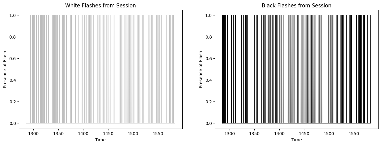
Next, we retrieve the stimulus information (full-field flashes) from the dataset.
To ensure they have a regular timescale, they are interpolated. Set bin_sz to be the bin size used for the interpolation below. Since bin_sz affects the temporal resolution of spikes and stimulus, bin_sz might have a large impact on the runtime and the performance of the model. This is because given a filer length in seconds, the bin size determines how many weights the filter consists of. More weights might may improve the performance of the GLM but will increase the runtime.
The stimulus information are stored in a series of tables, one of which is the flashes presentations table. In this table, the black and white flash intervals are listed with their respective start times and stop times, where -1.0 (black) and 1.0 (white) encode the color. Between these intervals, the screen was grey. The code below extracts these flash intervals and generates the interpolated flashes array.
There are several types of stimulus from this experimental session, but for the purposes of this analysis only the (approx.) 300 seconds of flashes stimulus are used.
bin_sz = 0.050 # important for performance of GLM, be careful!
flashes_table = nwb.intervals["flashes_presentations"]
flashes_table[:10]
| start_time | stop_time | stimulus_name | stimulus_block | color | mask | opacity | phase | size | units | stimulus_index | orientation | spatial_frequency | contrast | tags | timeseries | |
|---|---|---|---|---|---|---|---|---|---|---|---|---|---|---|---|---|
| id | ||||||||||||||||
| 0 | 1285.60087 | 1285.851080 | flashes | 1.0 | -1.0 | None | 1.0 | [0.0, 0.0] | [300.0, 300.0] | deg | 1.0 | 0.0 | [0.0, 0.0] | 0.8 | [stimulus_time_interval] | [(3647, 1, timestamps pynwb.base.TimeSeries at... |
| 1 | 1287.60256 | 1287.852768 | flashes | 1.0 | -1.0 | None | 1.0 | [0.0, 0.0] | [300.0, 300.0] | deg | 1.0 | 0.0 | [0.0, 0.0] | 0.8 | [stimulus_time_interval] | [(3648, 1, timestamps pynwb.base.TimeSeries at... |
| 2 | 1289.60423 | 1289.854435 | flashes | 1.0 | -1.0 | None | 1.0 | [0.0, 0.0] | [300.0, 300.0] | deg | 1.0 | 0.0 | [0.0, 0.0] | 0.8 | [stimulus_time_interval] | [(3649, 1, timestamps pynwb.base.TimeSeries at... |
| 3 | 1291.60589 | 1291.856100 | flashes | 1.0 | -1.0 | None | 1.0 | [0.0, 0.0] | [300.0, 300.0] | deg | 1.0 | 0.0 | [0.0, 0.0] | 0.8 | [stimulus_time_interval] | [(3650, 1, timestamps pynwb.base.TimeSeries at... |
| 4 | 1293.60761 | 1293.857808 | flashes | 1.0 | 1.0 | None | 1.0 | [0.0, 0.0] | [300.0, 300.0] | deg | 1.0 | 0.0 | [0.0, 0.0] | 0.8 | [stimulus_time_interval] | [(3651, 1, timestamps pynwb.base.TimeSeries at... |
| 5 | 1295.60925 | 1295.859455 | flashes | 1.0 | -1.0 | None | 1.0 | [0.0, 0.0] | [300.0, 300.0] | deg | 1.0 | 0.0 | [0.0, 0.0] | 0.8 | [stimulus_time_interval] | [(3652, 1, timestamps pynwb.base.TimeSeries at... |
| 6 | 1297.61096 | 1297.861155 | flashes | 1.0 | 1.0 | None | 1.0 | [0.0, 0.0] | [300.0, 300.0] | deg | 1.0 | 0.0 | [0.0, 0.0] | 0.8 | [stimulus_time_interval] | [(3653, 1, timestamps pynwb.base.TimeSeries at... |
| 7 | 1299.61265 | 1299.862843 | flashes | 1.0 | 1.0 | None | 1.0 | [0.0, 0.0] | [300.0, 300.0] | deg | 1.0 | 0.0 | [0.0, 0.0] | 0.8 | [stimulus_time_interval] | [(3654, 1, timestamps pynwb.base.TimeSeries at... |
| 8 | 1301.61429 | 1301.864488 | flashes | 1.0 | 1.0 | None | 1.0 | [0.0, 0.0] | [300.0, 300.0] | deg | 1.0 | 0.0 | [0.0, 0.0] | 0.8 | [stimulus_time_interval] | [(3655, 1, timestamps pynwb.base.TimeSeries at... |
| 9 | 1303.61592 | 1303.866128 | flashes | 1.0 | -1.0 | None | 1.0 | [0.0, 0.0] | [300.0, 300.0] | deg | 1.0 | 0.0 | [0.0, 0.0] | 0.8 | [stimulus_time_interval] | [(3656, 1, timestamps pynwb.base.TimeSeries at... |
start_time = np.min(flashes_table.start_time)
end_time = np.max(flashes_table.stop_time)
time_axis = np.linspace(start_time, end_time, num=int((end_time-start_time)//bin_sz), endpoint=False)

print("start:",start_time,"end:",end_time)
print(len(time_axis))

white_flashes = np.zeros(len(time_axis))
black_flashes = np.zeros(len(time_axis))
table_idx = 0
for i, ts in enumerate(time_axis):
    if ts > flashes_table.start_time[table_idx] and ts < flashes_table.stop_time[table_idx]:
        if float(flashes_table.color[table_idx]) == 1.0:
            white_flashes[i] = 1.0
        if float(flashes_table.color[table_idx]) == -1.0:
            black_flashes[i] = 1.0
    elif ts < flashes_table.start_time[table_idx]:
        continue
    while ts > flashes_table.stop_time[table_idx]:
        table_idx += 1

fig, axes = plt.subplots(1,2, figsize=(15,5))
axes[0].plot(time_axis, white_flashes, color="silver")
axes[0].set_title("White Flashes from Session")
axes[0].set_xlabel("Time")
axes[0].set_ylabel("Presence of Flash")

axes[1].plot(time_axis, black_flashes, color="black")
axes[1].set_title("Black Flashes from Session")
axes[1].set_xlabel("Time")
axes[1].set_ylabel("Presence of Flash")
start: 1285.6008699215513 end: 1584.1002475386938
5969
Text(0, 0.5, 'Presence of Flash')
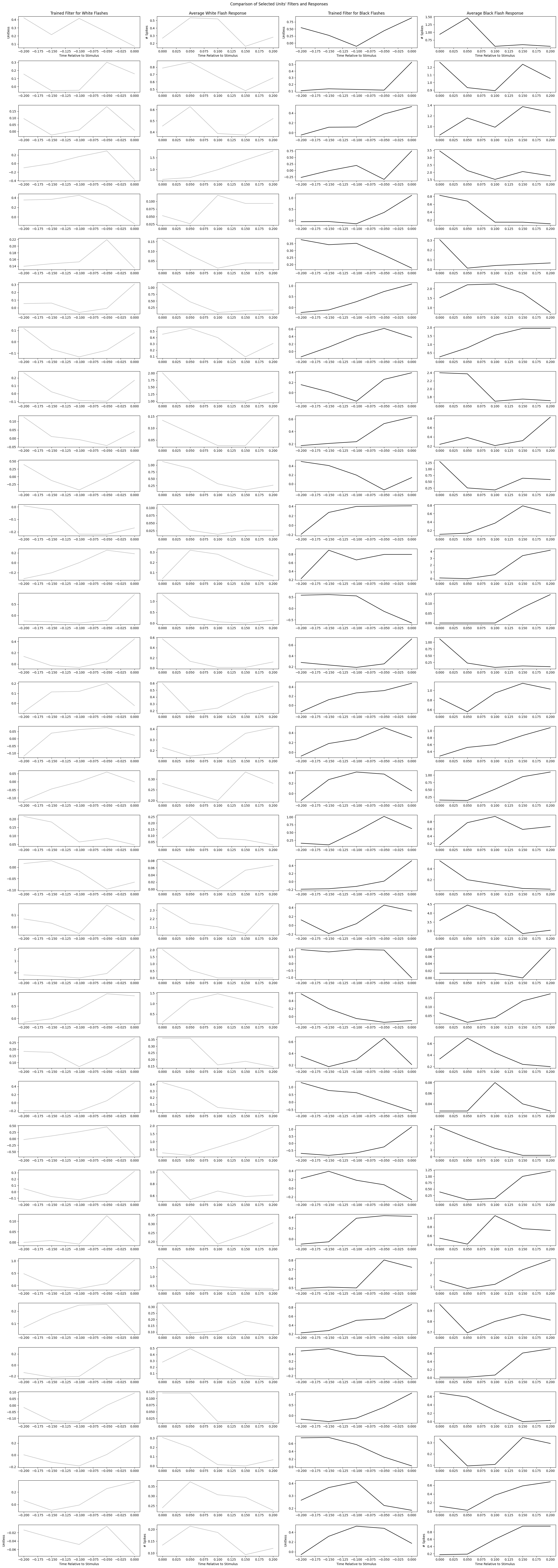
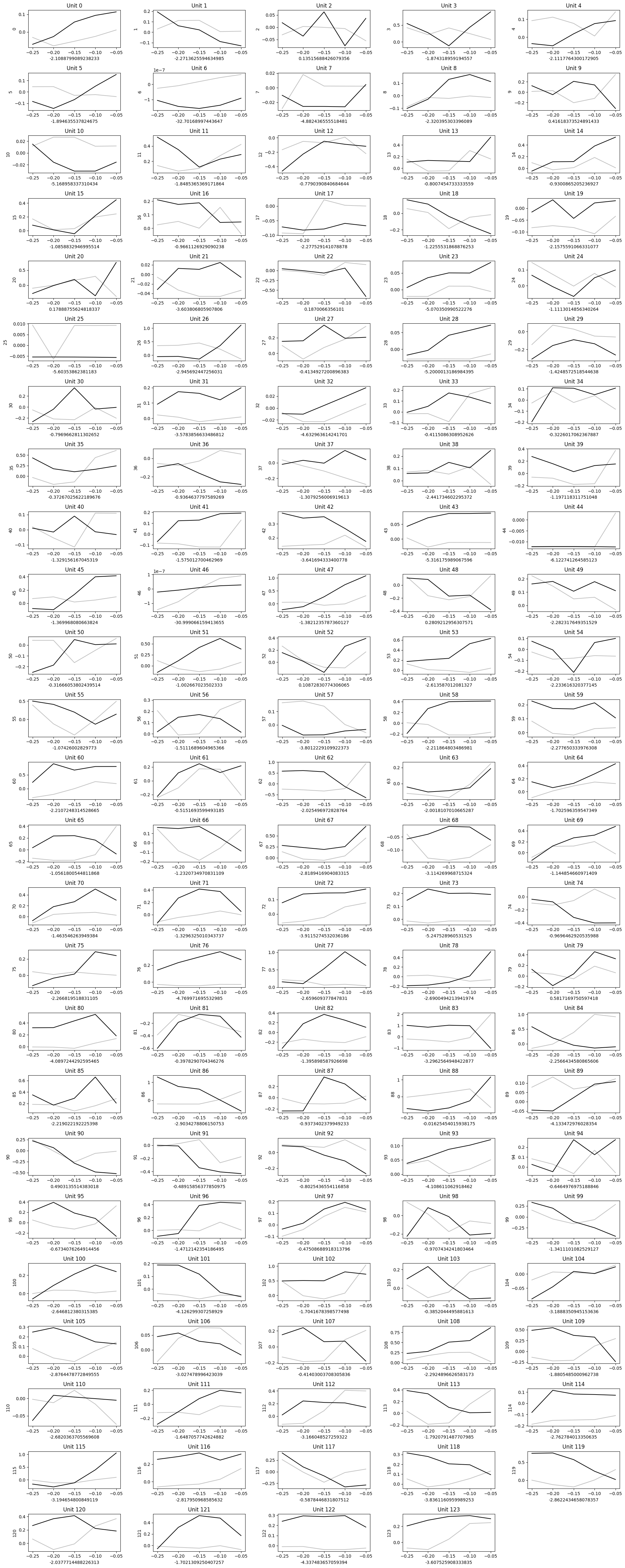
Generating Filters#
As with the synthetic data above, the design matrix is generated from the stimulus flashes. The filter length is set to 250 ms. Then, we train a GLM filter for each unit.
filter_duration = 0.250 # we want a 200 ms window,
filter_length = int(filter_duration / bin_sz) # divide by bin size to yield length of filter
filter_time_bins = np.linspace(-filter_duration, 0, filter_length+1, endpoint=True)

white_design_mat = build_design_mat(white_flashes, d=filter_length)
black_design_mat = build_design_mat(black_flashes, d=filter_length, include_const=False)
comb_design_mat = np.concatenate((white_design_mat, black_design_mat), axis=1)

print(white_design_mat.shape)
print(black_design_mat.shape)
print(comb_design_mat.shape)

# plt.imshow(comb_design_mat[:1000], extent=[-comb_design_mat.shape[1], 0, 1000, 0], aspect="auto", interpolation="none")
plt.imshow(comb_design_mat[:1000], aspect="auto", interpolation="none")
xaxis_step = 1
xpositions = range(0,comb_design_mat.shape[1])[::xaxis_step]
time_offset_axis = range(0, -comb_design_mat.shape[1]//2+1, -1)
xticks = ( ["und"] + list(time_offset_axis) + list(time_offset_axis))[::xaxis_step]

print(xpositions)
print(xticks)
plt.xticks(xpositions, xticks)
plt.xlabel("Time (bins prior to current)")
plt.ylabel("Current Time (bins through session)")
plt.title("Stimulus Design Matrix with Constant Column")
(5969, 6)
(5969, 5)
(5969, 11)
range(0, 11)
['und', 0, -1, -2, -3, -4, 0, -1, -2, -3, -4]
Text(0.5, 1.0, 'Stimulus Design Matrix with Constant Column')
training_outputs = []
for i, spike_times in enumerate(units_spike_times):
    # bin spikes where bins line up with the interpolated flashes timestamps
    these_spikes_binned, _ = np.histogram(spike_times, bins=len(time_axis), range=(start_time,end_time))
    # try:
    res = fit_lnp(comb_design_mat, these_spikes_binned, lam=2**5)
    midpoint = len(res)//2 + 1 # assumes the design mat has odd length
    const = res[0]
    white_filt = res[1:midpoint]
    black_filt = res[midpoint:]
    training_outputs.append((these_spikes_binned, const, white_filt, black_filt))
    # except:
    #     training_outputs.append((these_spikes_binned, np.nan, [], np.nan, []))
y: (5969,) X: (5969, 11) x0: (11,)
y: (5969,) X: (5969, 11) x0: (11,)
y: (5969,) X: (5969, 11) x0: (11,)
y: (5969,) X: (5969, 11) x0: (11,)
y: (5969,) X: (5969, 11) x0: (11,)
y: (5969,) X: (5969, 11) x0: (11,)
y: (5969,) X: (5969, 11) x0: (11,)
y: (5969,) X: (5969, 11) x0: (11,)
y: (5969,) X: (5969, 11) x0: (11,)
y: (5969,) X: (5969, 11) x0: (11,)
y: (5969,) X: (5969, 11) x0: (11,)
y: (5969,) X: (5969, 11) x0: (11,)
y: (5969,) X: (5969, 11) x0: (11,)
y: (5969,) X: (5969, 11) x0: (11,)
y: (5969,) X: (5969, 11) x0: (11,)
y: (5969,) X: (5969, 11) x0: (11,)
y: (5969,) X: (5969, 11) x0: (11,)
y: (5969,) X: (5969, 11) x0: (11,)
y: (5969,) X: (5969, 11) x0: (11,)
y: (5969,) X: (5969, 11) x0: (11,)
y: (5969,) X: (5969, 11) x0: (11,)
y: (5969,) X: (5969, 11) x0: (11,)
y: (5969,) X: (5969, 11) x0: (11,)
y: (5969,) X: (5969, 11) x0: (11,)
y: (5969,) X: (5969, 11) x0: (11,)
y: (5969,) X: (5969, 11) x0: (11,)
y: (5969,) X: (5969, 11) x0: (11,)
y: (5969,) X: (5969, 11) x0: (11,)
y: (5969,) X: (5969, 11) x0: (11,)
y: (5969,) X: (5969, 11) x0: (11,)
y: (5969,) X: (5969, 11) x0: (11,)
y: (5969,) X: (5969, 11) x0: (11,)
y: (5969,) X: (5969, 11) x0: (11,)
y: (5969,) X: (5969, 11) x0: (11,)
y: (5969,) X: (5969, 11) x0: (11,)
y: (5969,) X: (5969, 11) x0: (11,)
y: (5969,) X: (5969, 11) x0: (11,)
y: (5969,) X: (5969, 11) x0: (11,)
y: (5969,) X: (5969, 11) x0: (11,)
y: (5969,) X: (5969, 11) x0: (11,)
y: (5969,) X: (5969, 11) x0: (11,)
y: (5969,) X: (5969, 11) x0: (11,)
y: (5969,) X: (5969, 11) x0: (11,)
y: (5969,) X: (5969, 11) x0: (11,)
y: (5969,) X: (5969, 11) x0: (11,)
y: (5969,) X: (5969, 11) x0: (11,)
y: (5969,) X: (5969, 11) x0: (11,)
y: (5969,) X: (5969, 11) x0: (11,)
y: (5969,) X: (5969, 11) x0: (11,)
y: (5969,) X: (5969, 11) x0: (11,)
y: (5969,) X: (5969, 11) x0: (11,)
y: (5969,) X: (5969, 11) x0: (11,)
y: (5969,) X: (5969, 11) x0: (11,)
y: (5969,) X: (5969, 11) x0: (11,)
y: (5969,) X: (5969, 11) x0: (11,)
y: (5969,) X: (5969, 11) x0: (11,)
y: (5969,) X: (5969, 11) x0: (11,)
y: (5969,) X: (5969, 11) x0: (11,)
y: (5969,) X: (5969, 11) x0: (11,)
y: (5969,) X: (5969, 11) x0: (11,)
y: (5969,) X: (5969, 11) x0: (11,)
y: (5969,) X: (5969, 11) x0: (11,)
y: (5969,) X: (5969, 11) x0: (11,)
y: (5969,) X: (5969, 11) x0: (11,)
y: (5969,) X: (5969, 11) x0: (11,)
y: (5969,) X: (5969, 11) x0: (11,)
y: (5969,) X: (5969, 11) x0: (11,)
y: (5969,) X: (5969, 11) x0: (11,)
y: (5969,) X: (5969, 11) x0: (11,)
y: (5969,) X: (5969, 11) x0: (11,)
y: (5969,) X: (5969, 11) x0: (11,)
y: (5969,) X: (5969, 11) x0: (11,)
y: (5969,) X: (5969, 11) x0: (11,)
y: (5969,) X: (5969, 11) x0: (11,)
y: (5969,) X: (5969, 11) x0: (11,)
y: (5969,) X: (5969, 11) x0: (11,)
y: (5969,) X: (5969, 11) x0: (11,)
y: (5969,) X: (5969, 11) x0: (11,)
y: (5969,) X: (5969, 11) x0: (11,)
y: (5969,) X: (5969, 11) x0: (11,)
y: (5969,) X: (5969, 11) x0: (11,)
y: (5969,) X: (5969, 11) x0: (11,)
y: (5969,) X: (5969, 11) x0: (11,)
y: (5969,) X: (5969, 11) x0: (11,)
y: (5969,) X: (5969, 11) x0: (11,)
y: (5969,) X: (5969, 11) x0: (11,)
y: (5969,) X: (5969, 11) x0: (11,)
y: (5969,) X: (5969, 11) x0: (11,)
y: (5969,) X: (5969, 11) x0: (11,)
y: (5969,) X: (5969, 11) x0: (11,)
y: (5969,) X: (5969, 11) x0: (11,)
y: (5969,) X: (5969, 11) x0: (11,)
y: (5969,) X: (5969, 11) x0: (11,)
y: (5969,) X: (5969, 11) x0: (11,)
y: (5969,) X: (5969, 11) x0: (11,)
y: (5969,) X: (5969, 11) x0: (11,)
y: (5969,) X: (5969, 11) x0: (11,)
y: (5969,) X: (5969, 11) x0: (11,)
y: (5969,) X: (5969, 11) x0: (11,)
y: (5969,) X: (5969, 11) x0: (11,)
y: (5969,) X: (5969, 11) x0: (11,)
y: (5969,) X: (5969, 11) x0: (11,)
y: (5969,) X: (5969, 11) x0: (11,)
y: (5969,) X: (5969, 11) x0: (11,)
y: (5969,) X: (5969, 11) x0: (11,)
y: (5969,) X: (5969, 11) x0: (11,)
y: (5969,) X: (5969, 11) x0: (11,)
y: (5969,) X: (5969, 11) x0: (11,)
y: (5969,) X: (5969, 11) x0: (11,)
y: (5969,) X: (5969, 11) x0: (11,)
y: (5969,) X: (5969, 11) x0: (11,)
y: (5969,) X: (5969, 11) x0: (11,)
y: (5969,) X: (5969, 11) x0: (11,)
y: (5969,) X: (5969, 11) x0: (11,)
y: (5969,) X: (5969, 11) x0: (11,)
y: (5969,) X: (5969, 11) x0: (11,)
y: (5969,) X: (5969, 11) x0: (11,)
y: (5969,) X: (5969, 11) x0: (11,)
y: (5969,) X: (5969, 11) x0: (11,)
y: (5969,) X: (5969, 11) x0: (11,)
y: (5969,) X: (5969, 11) x0: (11,)
y: (5969,) X: (5969, 11) x0: (11,)
y: (5969,) X: (5969, 11) x0: (11,)
y: (5969,) X: (5969, 11) x0: (11,)
n_cols=5

n_rows = ceil(len(training_outputs)/n_cols)
fig, axes = plt.subplots(n_rows, n_cols, figsize=(20,2*n_rows))
if len(axes.shape) == 1:
    axes = axes.reshape((1, axes.shape[0]))

for i, ax in enumerate(axes.flatten()):
    if i >= len(training_outputs):
        ax.set_visible(False)
        continue
    _, const, white_filt, black_filt = training_outputs[i]
    ax.plot(filter_time_bins[:-1], white_filt, color="silver")
    ax.plot(filter_time_bins[:-1], black_filt, color="black")
    ax.set_ylabel(i)
    ax.set_xlabel(const)
    ax.set_title(f"Unit {i}")

fig.tight_layout()
plt.show()
Predict Activity#
Finally, these trained filters can be applied to the stimulus to generate predicted spiking probability and predicted spike counts. In a real use case, one could provide some hypothetical stimulus values to predict how the units of interest may respond. Note that since the Poisson generation is non-deterministic, the predicted spikes will differ with each run. To evaluate the GLM’s performance, the \(R^2\) values are calculated between the observed spikes and the predicted spike probability. Note that in the \(R^2\) distributions below, performance is higher for predicting black flashes.
prediction_outputs = []
for spikes_binned, constant, white_filter, black_filter in training_outputs:
    print(white_filter.shape)
    white_predicted_rate = predict(white_design_mat[:,1:], white_filter, constant)
    white_spikes_predicted = predict_spikes(white_design_mat[:,1:], white_filter, constant)
    white_r2 = r2_score(spikes_binned, white_predicted_rate)

    black_predicted_rate = predict(black_design_mat, black_filter, constant)
    black_spikes_predicted = predict_spikes(black_design_mat, black_filter, constant)
    black_r2 = r2_score(spikes_binned, black_predicted_rate)

    print("===")
    print("white observed mean rate:", np.sum(spikes_binned) / len(spikes_binned))
    print("white predicted mean rate:", np.sum(white_spikes_predicted) / len(white_spikes_predicted))
    print("white loss:",white_r2)
    print("black observed mean rate:", np.sum(spikes_binned) / len(spikes_binned))
    print("black predicted mean rate:", np.sum(black_spikes_predicted) / len(black_spikes_predicted))
    print("black loss:",black_r2)

    prediction_outputs.append([white_predicted_rate, white_spikes_predicted, white_r2, black_predicted_rate, black_spikes_predicted, black_r2])

white_r2s = np.array([output[2] for output in prediction_outputs])
black_r2s = np.array([output[5] for output in prediction_outputs])
print("==================")
print("average white loss:",np.mean(white_r2s))
print("average black loss:",np.mean(black_r2s))
(5,)
===
white observed mean rate: 0.1216284134695929
white predicted mean rate: 0.11626738147093316
white loss: 0.0003848557093315552
black observed mean rate: 0.1216284134695929
black predicted mean rate: 0.12196347796950913
black loss: 0.0011426315366189765
(5,)
===
white observed mean rate: 0.10571284972357178
white predicted mean rate: 0.1018596079745351
white loss: 0.0009655136229619332
black observed mean rate: 0.10571284972357178
black predicted mean rate: 0.1038699949740325
black loss: 0.0017283559296648043
(5,)
===
white observed mean rate: 1.139051767465237
white predicted mean rate: 1.1470933154632266
white loss: 0.0003733266939996982
black observed mean rate: 1.139051767465237
black predicted mean rate: 1.140392025464902
black loss: 0.0003282379855058526
(5,)
===
white observed mean rate: 0.2186295861953426
white predicted mean rate: 0.18311274920422183
white loss: 0.017914792592427897
black observed mean rate: 0.2186295861953426
black predicted mean rate: 0.19467247445133187
black loss: 0.07174470984217507
(5,)
===
white observed mean rate: 0.1256491874685877
white predicted mean rate: 0.12799463896800134
white loss: 0.0014413843598259923
black observed mean rate: 0.1256491874685877
black predicted mean rate: 0.1127492042218127
black loss: 0.00028849785661355654
(5,)
===
white observed mean rate: 0.14977383146255654
white predicted mean rate: 0.1573127827106718
white loss: 0.0002254654068708506
black observed mean rate: 0.14977383146255654
black predicted mean rate: 0.1542972022114257
black loss: 0.0018114592982365618
(5,)
===
white observed mean rate: 0.0
white predicted mean rate: 0.0
white loss: 0.0
black observed mean rate: 0.0
black predicted mean rate: 0.0
black loss: 0.0
(5,)
===
white observed mean rate: 0.007538951248115262
white predicted mean rate: 0.008376612497905847
white loss: 1.9006137864652217e-05
black observed mean rate: 0.007538951248115262
black predicted mean rate: 0.007371418998157145
black loss: 3.559776082862065e-05
(5,)
===
white observed mean rate: 0.09951415647512146
white predicted mean rate: 0.10051934997487016
white loss: 0.00012236392701803211
black observed mean rate: 0.09951415647512146
black predicted mean rate: 0.10437259172390685
black loss: 0.0012923085627645214
(5,)
===
white observed mean rate: 1.5391187803652202
white predicted mean rate: 1.5056123303735969
white loss: 0.019236524868015192
black observed mean rate: 1.5391187803652202
black predicted mean rate: 1.501591556374602
black loss: 0.028437051031692584
(5,)
===
white observed mean rate: 0.005696096498575976
white predicted mean rate: 0.005193499748701625
white loss: 4.3188527518500663e-05
black observed mean rate: 0.005696096498575976
black predicted mean rate: 0.005696096498575976
black loss: 5.690326573304372e-05
(5,)
===
white observed mean rate: 0.19852571620036857
white predicted mean rate: 0.1732283464566929
white loss: 0.008166714076554227
black observed mean rate: 0.19852571620036857
black predicted mean rate: 0.18529066845367734
black loss: 0.034702631204931
(5,)
===
white observed mean rate: 0.4265371083933657
white predicted mean rate: 0.44446305913888423
white loss: 0.004227828472543882
black observed mean rate: 0.4265371083933657
black predicted mean rate: 0.43893449489026637
black loss: 0.01875042856890119
(5,)
===
white observed mean rate: 0.508460378622885
white predicted mean rate: 0.4563578488859105
white loss: 0.004596785173297535
black observed mean rate: 0.508460378622885
black predicted mean rate: 0.4922097503769476
black loss: 0.051307099358714026
(5,)
===
white observed mean rate: 0.446976042888256
white predicted mean rate: 0.40107220639973196
white loss: -0.004926347130385089
black observed mean rate: 0.446976042888256
black predicted mean rate: 0.4657396548835651
black loss: 0.10049793706306276
(5,)
===
white observed mean rate: 0.37510470765622383
white predicted mean rate: 0.3590216116602446
white loss: 0.007595478119929999
black observed mean rate: 0.37510470765622383
black predicted mean rate: 0.3576813536605797
black loss: 0.017200694801386862
(5,)
===
white observed mean rate: 0.40593064164851733
white predicted mean rate: 0.37778522365555367
white loss: -5.138595963272152e-05
black observed mean rate: 0.40593064164851733
black predicted mean rate: 0.4106215446473446
black loss: 0.00612070655196062
(5,)
===
white observed mean rate: 0.09951415647512146
white predicted mean rate: 0.10303233372424192
white loss: 0.00039091941474289627
black observed mean rate: 0.09951415647512146
black predicted mean rate: 0.09700117272574971
black loss: 0.0008338045089394397
(5,)
===
white observed mean rate: 0.2888255989277936
white predicted mean rate: 0.2896632601775842
white loss: 0.0008306778729324504
black observed mean rate: 0.2888255989277936
black predicted mean rate: 0.2958619534260345
black loss: 0.00269197876065308
(5,)
===
white observed mean rate: 0.11341933322164517
white predicted mean rate: 0.10906349472273412
white loss: 0.0007623255694491071
black observed mean rate: 0.11341933322164517
black predicted mean rate: 0.12045568771988607
black loss: 5.151272924341921e-05
(5,)
===
white observed mean rate: 1.2373931981906516
white predicted mean rate: 1.1871335232032165
white loss: 0.008035544574526932
black observed mean rate: 1.2373931981906516
black predicted mean rate: 1.236388004690903
black loss: 0.05996413104523912
(5,)
===
white observed mean rate: 0.026972692243256827
white predicted mean rate: 0.02730775674317306
white loss: 8.655361853615595e-05
black observed mean rate: 0.026972692243256827
black predicted mean rate: 0.028648014742837995
black loss: 2.1777117094501364e-05
(5,)
===
white observed mean rate: 1.187636119953091
white predicted mean rate: 1.2432568269391857
white loss: 0.006454214102642908
black observed mean rate: 1.187636119953091
black predicted mean rate: 1.1769140559557716
black loss: 0.019201846553171587
(5,)
===
white observed mean rate: 0.0063662254984084435
white predicted mean rate: 0.006868822248282795
white loss: 2.168089848897381e-05
black observed mean rate: 0.0063662254984084435
black predicted mean rate: 0.005696096498575976
black loss: 0.000321451051522037
(5,)
===
white observed mean rate: 0.3387502094153124
white predicted mean rate: 0.34159825766460045
white loss: 0.002320225293207301
black observed mean rate: 0.3387502094153124
black predicted mean rate: 0.3384151449153962
black loss: 0.0005628944396857127
(5,)
===
white observed mean rate: 0.0036857094990785724
white predicted mean rate: 0.0041883062489529235
white loss: 8.387496791883997e-06
black observed mean rate: 0.0036857094990785724
black predicted mean rate: 0.00217791924945552
black loss: 3.3283996927480075e-06
(5,)
===
white observed mean rate: 0.06868822248282794
white predicted mean rate: 0.05830122298542469
white loss: 0.016620134991759072
black observed mean rate: 0.06868822248282794
black predicted mean rate: 0.061149271234712685
black loss: 0.036149389630828366
(5,)
===
white observed mean rate: 0.7626068018093483
white predicted mean rate: 0.6766627575808343
white loss: 0.007194643423468872
black observed mean rate: 0.7626068018093483
black predicted mean rate: 0.7257497068185625
black loss: 0.046566331382891235
(5,)
===
white observed mean rate: 0.005528564248617859
white predicted mean rate: 0.00603116099849221
white loss: 7.900903933755199e-05
black observed mean rate: 0.005528564248617859
black predicted mean rate: 0.005361031998659742
black loss: 0.00025421727454244536
(5,)
===
white observed mean rate: 0.2275087954431228
white predicted mean rate: 0.23521527894119618
white loss: 0.00011571588748582329
black observed mean rate: 0.2275087954431228
black predicted mean rate: 0.23286982744178256
black loss: 0.004185549026593627
(5,)
===
white observed mean rate: 0.4357513821410621
white predicted mean rate: 0.4392695593901826
white loss: 0.005071780398373749
black observed mean rate: 0.4357513821410621
black predicted mean rate: 0.4523370748869157
black loss: 0.003937504405343906
(5,)
===
white observed mean rate: 0.029653208242586698
white predicted mean rate: 0.028312950242921762
white loss: -6.458462948844002e-05
black observed mean rate: 0.029653208242586698
black predicted mean rate: 0.03350644999162339
black loss: 0.0036879960668028122
(5,)
===
white observed mean rate: 0.009716870497570782
white predicted mean rate: 0.010554531747361368
white loss: 2.7724438046106137e-05
black observed mean rate: 0.009716870497570782
black predicted mean rate: 0.009884402747528899
black loss: 3.949293473026749e-05
(5,)
===
white observed mean rate: 0.6974367565756409
white predicted mean rate: 0.6731445803317139
white loss: 0.008859155883803704
black observed mean rate: 0.6974367565756409
black predicted mean rate: 0.6687887418328028
black loss: 0.01563537368842216
(5,)
===
white observed mean rate: 0.7331211258167197
white predicted mean rate: 0.7493717540626571
white loss: 0.0005195540380142916
black observed mean rate: 0.7331211258167197
black predicted mean rate: 0.7369743675657564
black loss: 0.006908389128369441
(5,)
===
white observed mean rate: 0.8116937510470765
white predicted mean rate: 0.7399899480650025
white loss: 0.03600261224027024
black observed mean rate: 0.8116937510470765
black predicted mean rate: 0.7788574300552856
black loss: 0.035600931425925464
(5,)
===
white observed mean rate: 0.37577483665605627
white predicted mean rate: 0.3916904004020774
white loss: 0.00013269112177083375
black observed mean rate: 0.37577483665605627
black predicted mean rate: 0.3690735466577316
black loss: 0.0074715385571892945
(5,)
===
white observed mean rate: 0.2663762774334059
white predicted mean rate: 0.2596749874350813
white loss: 0.00393518111512392
black observed mean rate: 0.2663762774334059
black predicted mean rate: 0.2802814541799296
black loss: 0.001082962858229508
(5,)
===
white observed mean rate: 0.09314793097671302
white predicted mean rate: 0.09029988272742503
white loss: 0.0007904312238266042
black observed mean rate: 0.09314793097671302
black predicted mean rate: 0.08946222147763444
black loss: 0.004349019904693829
(5,)
===
white observed mean rate: 0.31864633942033843
white predicted mean rate: 0.306584017423354
white loss: 0.007530997023826869
black observed mean rate: 0.31864633942033843
black predicted mean rate: 0.32266711341933324
black loss: 0.014221172855047537
(5,)
===
white observed mean rate: 0.2667113419333222
white predicted mean rate: 0.2717373094320657
white loss: 0.0009270823265001837
black observed mean rate: 0.2667113419333222
black predicted mean rate: 0.26922432568269394
black loss: 0.00018613974805381517
(5,)
===
white observed mean rate: 0.21326855419668286
white predicted mean rate: 0.19819065170045233
white loss: 0.0016485908703034458
black observed mean rate: 0.21326855419668286
black predicted mean rate: 0.21192829619701792
black loss: 0.00724375773585928
(5,)
===
white observed mean rate: 0.032501256491874686
white predicted mean rate: 0.0326687887418328
white loss: 0.002561330929999661
black observed mean rate: 0.032501256491874686
black predicted mean rate: 0.03015580499246105
black loss: 0.020399737262718043
(5,)
===
white observed mean rate: 0.005025967498743508
white predicted mean rate: 0.007538951248115262
white loss: 2.2711039360689966e-05
black observed mean rate: 0.005025967498743508
black predicted mean rate: 0.004858435248785391
black loss: 0.0007943845878219946
(5,)
===
white observed mean rate: 0.00217791924945552
white predicted mean rate: 0.0011727257497068187
white loss: 1.340942709371351e-05
black observed mean rate: 0.00217791924945552
black predicted mean rate: 0.003015580499246105
black loss: 1.6160863511638368e-05
(5,)
===
white observed mean rate: 0.27910872843022283
white predicted mean rate: 0.24091137543977215
white loss: -0.0005299131067735274
black observed mean rate: 0.27910872843022283
black predicted mean rate: 0.27575808343106045
black loss: 0.038992589644905595
(5,)
===
white observed mean rate: 0.0
white predicted mean rate: 0.0
white loss: 0.0
black observed mean rate: 0.0
black predicted mean rate: 0.0
black loss: 0.0
(5,)
===
white observed mean rate: 0.33757748366560564
white predicted mean rate: 0.24945552018763612
white loss: -0.013224882349350375
black observed mean rate: 0.33757748366560564
black predicted mean rate: 0.3302060646674485
black loss: 0.26487208568094
(5,)
===
white observed mean rate: 1.2727425029318145
white predicted mean rate: 1.3112749204221812
white loss: 0.009631569902985637
black observed mean rate: 1.2727425029318145
black predicted mean rate: 1.2858100184285475
black loss: 0.01916969131860391
(5,)
===
white observed mean rate: 0.111744010722064
white predicted mean rate: 0.11258167197185458
white loss: 0.002918174604072954
black observed mean rate: 0.111744010722064
black predicted mean rate: 0.10923102697269224
black loss: 0.006983091930748975
(5,)
===
white observed mean rate: 0.712012062321997
white predicted mean rate: 0.7354665773161334
white loss: 0.001770086281769112
black observed mean rate: 0.712012062321997
black predicted mean rate: 0.7155302395711174
black loss: 0.010483056914401767
(5,)
===
white observed mean rate: 0.4292176243926956
white predicted mean rate: 0.3541631764114592
white loss: -0.008391718616928445
black observed mean rate: 0.4292176243926956
black predicted mean rate: 0.43591891439102026
black loss: 0.18986787495173962
(5,)
===
white observed mean rate: 1.1960127324509968
white predicted mean rate: 1.138716702965321
white loss: 0.003139719226269322
black observed mean rate: 1.1960127324509968
black predicted mean rate: 1.189311442452672
black loss: 0.052245840083565254
(5,)
===
white observed mean rate: 0.0909700117272575
white predicted mean rate: 0.08041547997989613
white loss: -0.002808738133622146
black observed mean rate: 0.0909700117272575
black predicted mean rate: 0.08795443122801139
black loss: 0.07340013913830312
(5,)
===
white observed mean rate: 0.10537778522365555
white predicted mean rate: 0.10856089797285978
white loss: 0.0008422770834660698
black observed mean rate: 0.10537778522365555
black predicted mean rate: 0.10705310772323673
black loss: 0.0015322509397520667
(5,)
===
white observed mean rate: 0.38968001340258
white predicted mean rate: 0.35165019266208747
white loss: 0.011151250336941754
black observed mean rate: 0.38968001340258
black predicted mean rate: 0.36924107890768976
black loss: 0.051190540321267686
(5,)
===
white observed mean rate: 0.2412464399396884
white predicted mean rate: 0.236388004690903
white loss: 0.011764365499912999
black observed mean rate: 0.2412464399396884
black predicted mean rate: 0.23270229519182442
black loss: 0.004697187935071234
(5,)
===
white observed mean rate: 0.022784385994303904
white predicted mean rate: 0.025799966493550007
white loss: 0.002484279361625874
black observed mean rate: 0.022784385994303904
black predicted mean rate: 0.022784385994303904
black loss: 0.00031485311797696536
(5,)
===
white observed mean rate: 0.12280113921929972
white predicted mean rate: 0.10755570447311108
white loss: 0.0014719862613212786
black observed mean rate: 0.12280113921929972
black predicted mean rate: 0.12347126821913218
black loss: 0.058630585406477476
(5,)
===
white observed mean rate: 0.11124141397218965
white predicted mean rate: 0.09716870497570783
white loss: -0.0004295403760308236
black observed mean rate: 0.11124141397218965
black predicted mean rate: 0.10454012397386497
black loss: 0.010373524034677062
(5,)
===
white observed mean rate: 0.22482827944379294
white predicted mean rate: 0.11107388172223152
white loss: -0.020726940986139697
black observed mean rate: 0.22482827944379294
black predicted mean rate: 0.23421008544144747
black loss: 0.5274035051768187
(5,)
===
white observed mean rate: 0.6138381638465404
white predicted mean rate: 0.5950745518512314
white loss: 0.0038072560698744207
black observed mean rate: 0.6138381638465404
black predicted mean rate: 0.6161836153459541
black loss: 0.017373712868559044
(5,)
===
white observed mean rate: 0.15479979896130006
white predicted mean rate: 0.1325180097168705
white loss: 0.028725009902258125
black observed mean rate: 0.15479979896130006
black predicted mean rate: 0.15412966996146757
black loss: 0.10951727486789076
(5,)
===
white observed mean rate: 0.13318813871670296
white predicted mean rate: 0.13419333221645166
white loss: 0.0032526677027278073
black observed mean rate: 0.13318813871670296
black predicted mean rate: 0.14876863796280784
black loss: 0.0014937904135995383
(5,)
===
white observed mean rate: 0.2038867481990283
white predicted mean rate: 0.19551013570112247
white loss: -6.204172880952541e-05
black observed mean rate: 0.2038867481990283
black predicted mean rate: 0.20087116769978222
black loss: 0.023569761078984897
(5,)
===
white observed mean rate: 0.3628748534092813
white predicted mean rate: 0.3482995476629251
white loss: 0.008453908205621308
black observed mean rate: 0.3628748534092813
black predicted mean rate: 0.3613670631596582
black loss: 0.015485288268646369
(5,)
===
white observed mean rate: 0.30139051767465236
white predicted mean rate: 0.2925113084268722
white loss: 0.0020439999508167217
black observed mean rate: 0.30139051767465236
black predicted mean rate: 0.30541129167364717
black loss: 0.007643610458605288
(5,)
===
white observed mean rate: 0.07388172223152957
white predicted mean rate: 0.06047914223488021
white loss: 0.0020788155869526648
black observed mean rate: 0.07388172223152957
black predicted mean rate: 0.07136873848215781
black loss: 0.020099392222687973
(5,)
===
white observed mean rate: 0.042720723739319816
white predicted mean rate: 0.04020773998994807
white loss: 0.001247608968091396
black observed mean rate: 0.042720723739319816
black predicted mean rate: 0.04523370748869157
black loss: 0.00016570890840528207
(5,)
===
white observed mean rate: 0.3613670631596582
white predicted mean rate: 0.33372424191656896
white loss: -0.00048115737569398576
black observed mean rate: 0.3613670631596582
black predicted mean rate: 0.34980733791254814
black loss: 0.06249341928624785
(5,)
===
white observed mean rate: 0.26252303568436924
white predicted mean rate: 0.23622047244094488
white loss: -0.0028752364128576957
black observed mean rate: 0.26252303568436924
black predicted mean rate: 0.2579996649355001
black loss: 0.06313366049042235
(5,)
===
white observed mean rate: 0.28916066342770985
white predicted mean rate: 0.26721393868319654
white loss: -0.0013935124271227117
black observed mean rate: 0.28916066342770985
black predicted mean rate: 0.28949572792762607
black loss: 0.046019911569354144
(5,)
===
white observed mean rate: 0.021109063494722736
white predicted mean rate: 0.019433740995141564
white loss: 0.00022443187578335966
black observed mean rate: 0.021109063494722736
black predicted mean rate: 0.0217791924945552
black loss: 0.002958126869226807
(5,)
===
white observed mean rate: 0.005696096498575976
white predicted mean rate: 0.005025967498743508
white loss: -1.7133527077106692e-06
black observed mean rate: 0.005696096498575976
black predicted mean rate: 0.0031831127492042218
black loss: 0.006002598532940384
(5,)
===
white observed mean rate: 0.35583849891104036
white predicted mean rate: 0.3648852404087787
white loss: 0.00030375955412242917
black observed mean rate: 0.35583849891104036
black predicted mean rate: 0.3603618696599095
black loss: 0.018020993600989077
(5,)
===
white observed mean rate: 0.10772323672306919
white predicted mean rate: 0.09984922097503769
white loss: -7.948466588914016e-06
black observed mean rate: 0.10772323672306919
black predicted mean rate: 0.10671804322332049
black loss: 0.005971261495489433
(5,)
===
white observed mean rate: 0.009549338247612666
white predicted mean rate: 0.007036354498240911
white loss: 9.971134382613656e-07
black observed mean rate: 0.009549338247612666
black predicted mean rate: 0.013235047746691238
black loss: 0.01141134341316874
(5,)
===
white observed mean rate: 0.10738817222315296
white predicted mean rate: 0.07706483498073378
white loss: -0.00842491822652125
black observed mean rate: 0.10738817222315296
black predicted mean rate: 0.09834143072541464
black loss: 0.17831098868701056
(5,)
===
white observed mean rate: 0.0681856257329536
white predicted mean rate: 0.07103367398224159
white loss: 0.00039056734230424883
black observed mean rate: 0.0681856257329536
black predicted mean rate: 0.05863628748534093
black loss: 0.01146695862813174
(5,)
===
white observed mean rate: 1.946724744513319
white predicted mean rate: 1.8520690232869828
white loss: -0.004332975104232917
black observed mean rate: 1.946724744513319
black predicted mean rate: 1.8793767800301557
black loss: 0.11411576076738605
(5,)
===
white observed mean rate: 0.020941531244764618
white predicted mean rate: 0.018931144245267213
white loss: -0.00035844682468222366
black observed mean rate: 0.020941531244764618
black predicted mean rate: 0.0207739989948065
black loss: 0.0345472538917142
(5,)
===
white observed mean rate: 0.5979226001005193
white predicted mean rate: 0.6501926620874519
white loss: 0.022654840973459822
black observed mean rate: 0.5979226001005193
black predicted mean rate: 0.6393030658401743
black loss: 0.036152384220748846
(5,)
===
white observed mean rate: 0.25079577818730103
white predicted mean rate: 0.2422516334394371
white loss: 0.007698330657577079
black observed mean rate: 0.25079577818730103
black predicted mean rate: 0.26453342268386665
black loss: 0.02964700407652221
(5,)
===
white observed mean rate: 0.08761936672809516
white predicted mean rate: 0.04707656223823086
white loss: 0.03912638050163242
black observed mean rate: 0.08761936672809516
black predicted mean rate: 0.08343106047914224
black loss: 0.41661023549371845
(5,)
===
white observed mean rate: 0.15546992796113251
white predicted mean rate: 0.1553023957111744
white loss: 0.24071110804163243
black observed mean rate: 0.15546992796113251
black predicted mean rate: 0.1147595912213101
black loss: -0.003544069869673372
(5,)
===
white observed mean rate: 0.13938683196515328
white predicted mean rate: 0.11224660747193835
white loss: 0.0013094460554390341
black observed mean rate: 0.13938683196515328
black predicted mean rate: 0.13519852571620036
black loss: 0.0525031573351169
(5,)
===
white observed mean rate: 0.08577651197855587
white predicted mean rate: 0.05562070698609482
white loss: -0.0029877539877321
black observed mean rate: 0.08577651197855587
black predicted mean rate: 0.08376612497905847
black loss: 0.29527689638455723
(5,)
===
white observed mean rate: 0.38934494890266375
white predicted mean rate: 0.39001507790249623
white loss: 0.002426687535275418
black observed mean rate: 0.38934494890266375
black predicted mean rate: 0.40107220639973196
black loss: 0.01301334602588411
(5,)
===
white observed mean rate: 0.9991623387502094
white predicted mean rate: 1.0018428547495393
white loss: 0.037411280011980796
black observed mean rate: 0.9991623387502094
black predicted mean rate: 0.984251968503937
black loss: 0.18023503931300244
(5,)
===
white observed mean rate: 0.016753224995811694
white predicted mean rate: 0.014407773496398057
white loss: 0.0009836851823887827
black observed mean rate: 0.016753224995811694
black predicted mean rate: 0.01474283799631429
black loss: 0.0004074757637352322
(5,)
===
white observed mean rate: 1.5660914726084771
white predicted mean rate: 1.6195342603451164
white loss: 0.005582469816833413
black observed mean rate: 1.5660914726084771
black predicted mean rate: 1.5535265538616183
black loss: 0.03995618295001979
(5,)
===
white observed mean rate: 0.5719551013570112
white predicted mean rate: 0.6069693415982577
white loss: 0.004594055485344972
black observed mean rate: 0.5719551013570112
black predicted mean rate: 0.5910537778522366
black loss: 0.03570782522818294
(5,)
===
white observed mean rate: 0.4566929133858268
white predicted mean rate: 0.4726084771318479
white loss: 0.0050918068977100495
black observed mean rate: 0.4566929133858268
black predicted mean rate: 0.4439604623890099
black loss: 0.003264670411580739
(5,)
===
white observed mean rate: 0.017088289495727927
white predicted mean rate: 0.016920757245769812
white loss: 0.00012482945702541048
black observed mean rate: 0.017088289495727927
black predicted mean rate: 0.015412966996146759
black loss: 0.0010144683492098183
(5,)
===
white observed mean rate: 0.5575473278606131
white predicted mean rate: 0.531412296867147
white loss: -0.0002526171154308976
black observed mean rate: 0.5575473278606131
black predicted mean rate: 0.5397889093650527
black loss: 0.03682371257986805
(5,)
===
white observed mean rate: 0.5454850058636288
white predicted mean rate: 0.5267213938683196
white loss: 0.004374109598986542
black observed mean rate: 0.5454850058636288
black predicted mean rate: 0.5394538448651366
black loss: 0.05856601626317448
(5,)
===
white observed mean rate: 0.25950745518512314
white predicted mean rate: 0.23622047244094488
white loss: -0.0033081448092007193
black observed mean rate: 0.25950745518512314
black predicted mean rate: 0.25548668118612833
black loss: 0.07120280741004126
(5,)
===
white observed mean rate: 0.651867984587033
white predicted mean rate: 0.6238900988440275
white loss: 0.005406319718767927
black observed mean rate: 0.651867984587033
black predicted mean rate: 0.6394705980901324
black loss: 0.01753802380690017
(5,)
===
white observed mean rate: 0.36455017590886246
white predicted mean rate: 0.3858267716535433
white loss: 0.00284219726603685
black observed mean rate: 0.36455017590886246
black predicted mean rate: 0.3560060311609985
black loss: 0.008543525574980504
(5,)
===
white observed mean rate: 0.2636957614340761
white predicted mean rate: 0.2600100519349975
white loss: 0.005098600537176479
black observed mean rate: 0.2636957614340761
black predicted mean rate: 0.24476461718880885
black loss: 0.017924502576857182
(5,)
===
white observed mean rate: 0.07639470598090133
white predicted mean rate: 0.07354665773161334
white loss: -0.00029732467387688644
black observed mean rate: 0.07639470598090133
black predicted mean rate: 0.08091807672977049
black loss: 0.010869539238476
(5,)
===
white observed mean rate: 0.01641816049589546
white predicted mean rate: 0.016083095995979225
white loss: 0.00027707162775403305
black observed mean rate: 0.01641816049589546
black predicted mean rate: 0.019266208745183446
black loss: 0.002454003406159977
(5,)
===
white observed mean rate: 0.3407605964148098
white predicted mean rate: 0.21008544144747865
white loss: -0.010041782738266836
black observed mean rate: 0.3407605964148098
black predicted mean rate: 0.31093985592226503
black loss: 0.3267876990113304
(5,)
===
white observed mean rate: 0.7043055788239236
white predicted mean rate: 0.6883900150779025
white loss: 0.011774855836110487
black observed mean rate: 0.7043055788239236
black predicted mean rate: 0.67616016083096
black loss: 0.006270160914384704
(5,)
===
white observed mean rate: 0.04104540123973865
white predicted mean rate: 0.04640643323839839
white loss: 3.368799417646784e-05
black observed mean rate: 0.04104540123973865
black predicted mean rate: 0.04372591723906852
black loss: 0.00023014749457739292
(5,)
===
white observed mean rate: 0.06265706148433574
white predicted mean rate: 0.057966158485508464
white loss: 0.0001540282344231203
black observed mean rate: 0.06265706148433574
black predicted mean rate: 0.05428044898642989
black loss: 0.011985768878747805
(5,)
===
white observed mean rate: 0.049422013737644495
white predicted mean rate: 0.04824928798793768
white loss: 0.0004179848013005083
black observed mean rate: 0.049422013737644495
black predicted mean rate: 0.04875188473781203
black loss: 0.0001908145468917377
(5,)
===
white observed mean rate: 0.6736471770815882
white predicted mean rate: 0.6463394203384152
white loss: 0.0061140655907607755
black observed mean rate: 0.6736471770815882
black predicted mean rate: 0.6987770145753057
black loss: 0.011359336055889457
(5,)
===
white observed mean rate: 0.1521192829619702
white predicted mean rate: 0.10755570447311108
white loss: -0.008313439416093527
black observed mean rate: 0.1521192829619702
black predicted mean rate: 0.13804657396548836
black loss: 0.172227165391444
(5,)
===
white observed mean rate: 0.18210755570447312
white predicted mean rate: 0.15647512146088122
white loss: 0.0009569106488862555
black observed mean rate: 0.18210755570447312
black predicted mean rate: 0.1849556039537611
black loss: 0.10988971973614292
(5,)
===
white observed mean rate: 0.06785056123303736
white predicted mean rate: 0.07103367398224159
white loss: 0.00014871859627829664
black observed mean rate: 0.06785056123303736
black predicted mean rate: 0.06952588373261853
black loss: 9.119497109888464e-05
(5,)
===
white observed mean rate: 0.18931144245267215
white predicted mean rate: 0.189143910202714
white loss: 0.0023364392394086275
black observed mean rate: 0.18931144245267215
black predicted mean rate: 0.20723739319819065
black loss: 0.006056428710098816
(5,)
===
white observed mean rate: 0.04791422348802144
white predicted mean rate: 0.04339085273915229
white loss: 0.01064306978484253
black observed mean rate: 0.04791422348802144
black predicted mean rate: 0.04473111073881722
black loss: 0.006224699349372975
(5,)
===
white observed mean rate: 0.18261015245434747
white predicted mean rate: 0.16853744345786564
white loss: 0.006019444900695947
black observed mean rate: 0.18261015245434747
black predicted mean rate: 0.16853744345786564
black loss: 0.015814799955819137
(5,)
===
white observed mean rate: 0.061986932484503265
white predicted mean rate: 0.05377785223655554
white loss: 0.0023208338444413723
black observed mean rate: 0.061986932484503265
black predicted mean rate: 0.06349472273412632
black loss: 0.001124355702116664
(5,)
===
white observed mean rate: 0.04573630423856592
white predicted mean rate: 0.03819735299045066
white loss: 0.00021551674479525218
black observed mean rate: 0.04573630423856592
black predicted mean rate: 0.04540123973864969
black loss: 0.04577495452770619
(5,)
===
white observed mean rate: 0.06935835148266041
white predicted mean rate: 0.055285642486178586
white loss: -0.0006439349986779863
black observed mean rate: 0.06935835148266041
black predicted mean rate: 0.06919081923270229
black loss: 0.024787389770898116
(5,)
===
white observed mean rate: 0.5577148601105713
white predicted mean rate: 0.5649187468587703
white loss: 0.0042630699978698505
black observed mean rate: 0.5577148601105713
black predicted mean rate: 0.5525213603618696
black loss: 0.015539429275134964
(5,)
===
white observed mean rate: 0.02412464399396884
white predicted mean rate: 0.020941531244764618
white loss: 0.00023852470514440505
black observed mean rate: 0.02412464399396884
black predicted mean rate: 0.020606466744848385
black loss: 0.00970105028987478
(5,)
===
white observed mean rate: 0.083095995979226
white predicted mean rate: 0.0603116099849221
white loss: -0.004079967160372622
black observed mean rate: 0.083095995979226
black predicted mean rate: 0.08276093147930977
black loss: 0.13927174165931966
(5,)
===
white observed mean rate: 0.15798291171050427
white predicted mean rate: 0.13720891271569777
white loss: 0.004468796457906987
black observed mean rate: 0.15798291171050427
black predicted mean rate: 0.15764784721058803
black loss: 0.05556170180422659
(5,)
===
white observed mean rate: 0.21226336069693416
white predicted mean rate: 0.1829452169542637
white loss: -0.004248195821840994
black observed mean rate: 0.21226336069693416
black predicted mean rate: 0.21393868319651532
black loss: 0.10387382200167161
(5,)
===
white observed mean rate: 0.01474283799631429
white predicted mean rate: 0.01256491874685877
white loss: -0.00010849882499841534
black observed mean rate: 0.01474283799631429
black predicted mean rate: 0.011894789747026303
black loss: 0.015097436653518703
(5,)
===
white observed mean rate: 0.03216619199195845
white predicted mean rate: 0.025464901993633774
white loss: 0.0024342311859334442
black observed mean rate: 0.03216619199195845
black predicted mean rate: 0.03501424024124644
black loss: 0.020266324724482088
==================
average white loss: 0.004894024031872066
average black loss: 0.0412103108503236
fig, axes = plt.subplots(1,2, figsize=(15,5))

axes[0].hist(white_r2s, bins=100, color="silver")
axes[0].set_title("White Flashes Prediction $R^2s$")
axes[0].set_xlabel("$R^2$")
axes[0].set_ylabel("# Units")

axes[1].hist(black_r2s, bins=100, color="black")
axes[1].set_title("Black Flashes Prediction $R^2s$")
axes[1].set_xlabel("$R^2$")
axes[1].set_ylabel("# Units")
Text(0, 0.5, '# Units')
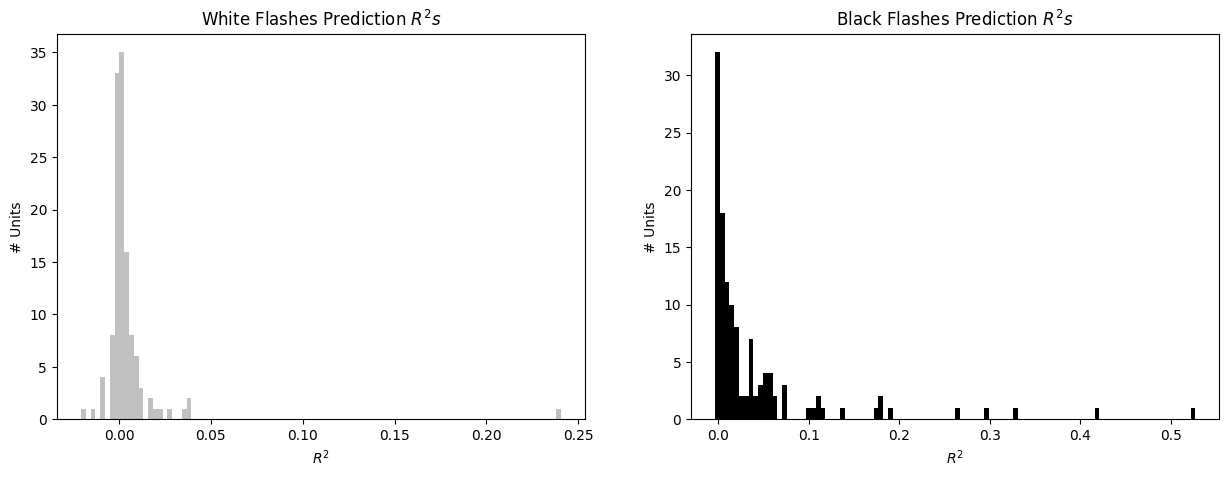
Showing Predictions#
Here, each model is plotted trained filter and prediction outputs. For ease of interpretation and to save space, only the best performing GLMs are displayed. This is done by selecting the prediction outputs with an \(R^2\) higher than 0.05. Model fitting is useful if you are expecting neuronal activity to follow a certain behavior. In the case of our Poisson model, we impose a certain response formula and fit the data to it. It can be sometimes useful to compare this fit with a more open-ended selection of cells: for instance, selecting cells simply based on whether the cell fired above a certain threshold. The combination of both approaches can allow to select cells to which fitting a model yield meaningful insights. In some cases, a non-responsive cell could provide model parameters that are hard to interpret. So it is always judicious to combine approaches.
In the first plot below, it can be seen that there is only one White Flashes model with an \(R^2\) greater than 0.05, indicating that in these data, units are less reliably responsive to white flashes than black. For each unit, real observed spikes given are shown, along with the trained model’s filter. Then the predicted spike rate, which as a reminder is the trained filter convolved over the input flashes. Finally, there is the predicted spikes which are the result of running the predicted spike rate through poisson generation. Because poisson is non-determinstic, these may look different every run.
white_best_fits = white_r2s > 0.05
white_best_training_outputs = np.array(training_outputs, dtype=object)[white_best_fits]
white_best_prediction_outputs = np.array(prediction_outputs, dtype=object)[white_best_fits]

black_best_fits = black_r2s > 0.05
black_best_training_outputs = np.array(training_outputs, dtype=object)[black_best_fits]
black_best_prediction_outputs = np.array(prediction_outputs, dtype=object)[black_best_fits]
n_cells = len(white_best_training_outputs)
fig, axes = plt.subplots(n_cells, 5, figsize=(30,2*n_cells+1))
if len(axes.shape) == 1:
    axes = np.expand_dims(axes, 0)

for i in range(len(white_best_training_outputs)):
    spikes_binned, constant, filter, _ = white_best_training_outputs[i]
    predicted_rate, spikes_predicted, r2, _, _, _ = white_best_prediction_outputs[i]

    time_range_start = 0
    time_range_end = 1000
    axes[i][0].plot(time_axis[time_range_start:time_range_end], spikes_binned[time_range_start:time_range_end])
    axes[i][1].plot(filter_time_bins[:-1], filter, color="crimson")
    axes[i][2].plot(time_axis[time_range_start:time_range_end], predicted_rate[time_range_start:time_range_end], color="indigo")
    axes[i][3].plot(time_axis[time_range_start:time_range_end], spikes_predicted[time_range_start:time_range_end], color="tab:orange")
    axes[i][4].plot(time_axis[time_range_start:time_range_end], spikes_binned[time_range_start:time_range_end])
    axes[i][4].plot(time_axis[time_range_start:time_range_end], spikes_predicted[time_range_start:time_range_end], color="tab:orange")

axes[0][0].set_title("Observed Spikes")
axes[0][1].set_title("Trained Filter")
axes[0][2].set_title("Predicted Spike Rate")
axes[0][3].set_title("Predicted Spikes")
axes[0][4].set_title("Observed Spikes (b) + Predicted Spikes (o)")
for ax_x, ax_y in ((0,0), (0,2), (0,3), (0,4), (-1,0), (-1,2), (-1,3), (-1,4)):
    axes[ax_x][ax_y].set_xlabel("Time throughout Session")
for ax_x, ax_y in ((0,1), (-1,1)):
    axes[ax_x][ax_y].set_xlabel("Time relative to Stimulus Event")

fig.suptitle("Best White Flashes Models", y=1, size=20)
fig.tight_layout()
plt.show()
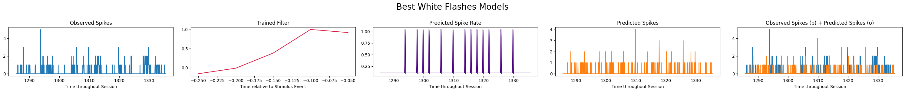
n_cells = len(black_best_training_outputs)
fig, axes = plt.subplots(n_cells, 5, figsize=(30,2*n_cells+1))
if len(axes.shape) == 1:
    axes = np.expand_dims(axes, 0)

for i in range(len(black_best_training_outputs)):
    spikes_binned, constant, _, filter = black_best_training_outputs[i]
    _, _, _, predicted_rate, spikes_predicted, r2 = black_best_prediction_outputs[i]

    time_range_start = 0
    time_range_end = 500
    axes[i][0].plot(time_axis[time_range_start:time_range_end], spikes_binned[time_range_start:time_range_end])
    axes[i][1].plot(filter_time_bins[:-1], filter, color="crimson")
    axes[i][2].plot(time_axis[time_range_start:time_range_end], predicted_rate[time_range_start:time_range_end], color="indigo")
    axes[i][3].plot(time_axis[time_range_start:time_range_end], spikes_predicted[time_range_start:time_range_end], color="tab:orange")
    axes[i][4].plot(time_axis[time_range_start:time_range_end], spikes_binned[time_range_start:time_range_end], alpha=0.8)
    axes[i][4].plot(time_axis[time_range_start:time_range_end], spikes_predicted[time_range_start:time_range_end], color="tab:orange", alpha=0.8)

axes[0][0].set_title("Observed Spikes")
axes[0][1].set_title("Trained Filter")
axes[0][2].set_title("Predicted Spike Rate")
axes[0][3].set_title("Predicted Spikes")
axes[0][4].set_title("Observed Spikes (b) + Predicted Spikes (o)")
for ax_x, ax_y in ((0,0), (0,2), (0,3), (0,4), (-1,0), (-1,2), (-1,3), (-1,4)):
    axes[ax_x][ax_y].set_xlabel("Time throughout Session")
for ax_x, ax_y in ((0,1), (-1,1)):
    axes[ax_x][ax_y].set_xlabel("Time relative to Stimulus Event")

fig.suptitle("Best Black Flashes Models", y=1, size=20)
fig.tight_layout()
plt.show()
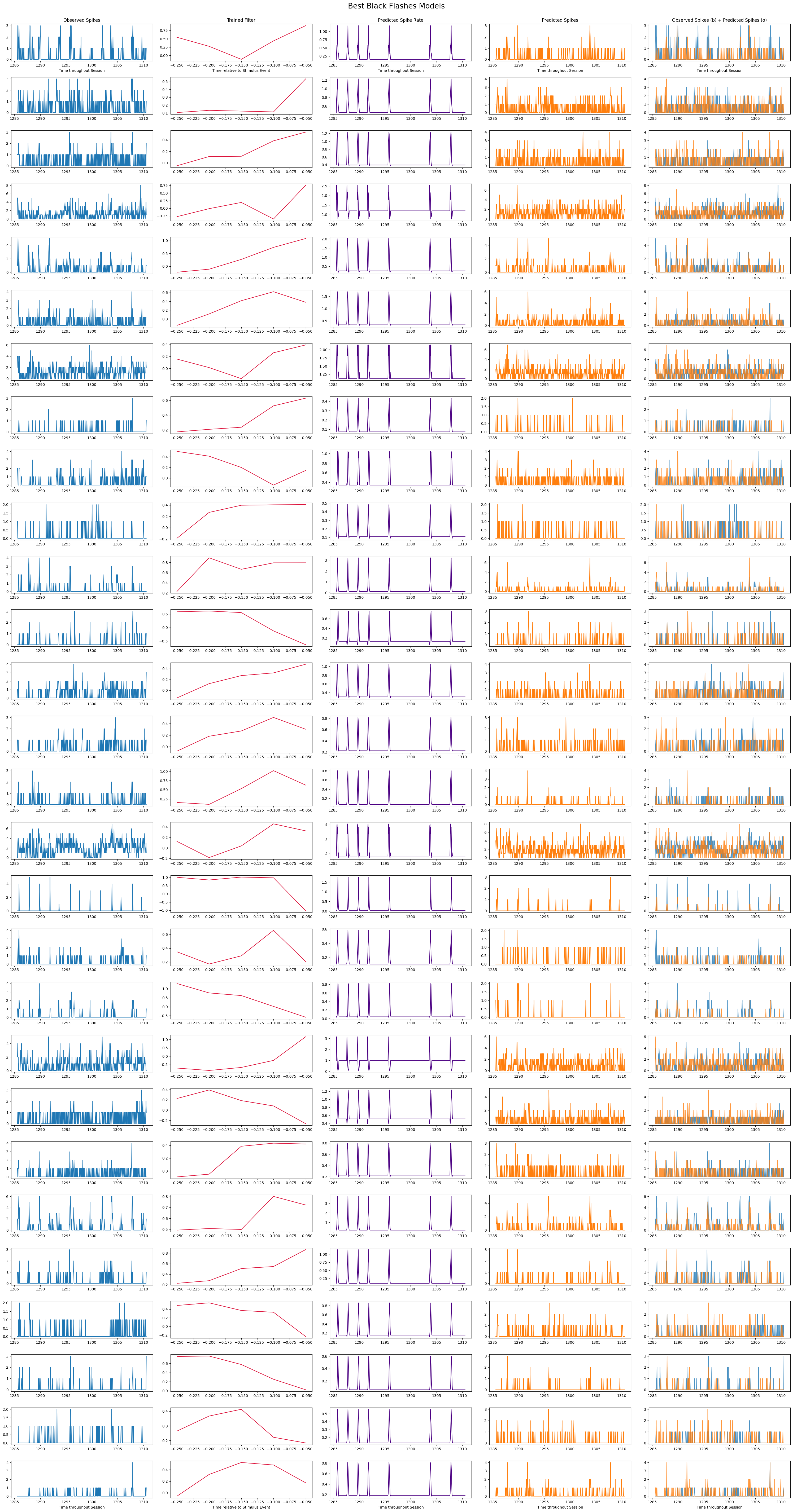
Comparing to Z-Scores#
# start and end times (relative to the stimulus at 0 seconds) that we want to examine and align spikes to
window_start_time = -(filter_length * bin_sz)
window_end_time = (filter_length * bin_sz)
def get_spike_matrix(stim_times, units_spike_times, bin_edges):
    time_resolution = np.mean(np.diff(bin_edges))
    # 3D spike matrix to be populated with spike counts
    spike_matrix = np.zeros((len(units_spike_times), len(stim_times), len(bin_edges)-1))

    # populate 3D spike matrix for each unit for each stimulus trial by counting spikes into bins
    for unit_idx in range(len(units_spike_times)):
        spike_times = units_spike_times[unit_idx]

        for stim_idx, stim_time in enumerate(stim_times):
            # get spike times that fall within the bin's time range relative to the stim time
            first_bin_time = stim_time + bin_edges[0]
            last_bin_time = stim_time + bin_edges[-1]
            first_spike_in_range, last_spike_in_range = np.searchsorted(spike_times, [first_bin_time, last_bin_time])
            spike_times_in_range = spike_times[first_spike_in_range:last_spike_in_range]

            # convert spike times into relative time bin indices
            bin_indices = ((spike_times_in_range - (first_bin_time)) / time_resolution).astype(int)

            # mark that there is a spike at these bin times for this unit on this stim trial
            for bin_idx in bin_indices:
                spike_matrix[unit_idx, stim_idx, bin_idx] += 1

    return spike_matrix
white_flash_times = time_axis[[i for i in range(1,len(white_flashes)) if white_flashes[i] == 1 and white_flashes[i-1] == 0]]
black_flash_times = time_axis[[i for i in range(1,len(black_flashes)) if black_flashes[i] == 1 and black_flashes[i-1] == 0]]

# time bins used
n_bins = int((window_end_time - window_start_time) / bin_sz)
bin_edges = np.linspace(window_start_time, window_end_time, n_bins+1, endpoint=True)
# bin_edges = np.concatenate((filter_time_bins, -filter_time_bins[:-1][::-1]))

# calculate baseline and stimulus interval indices for use later
stimulus_onset_idx = int(-bin_edges[0] / bin_sz)

white_flash_responses = get_spike_matrix(white_flash_times, units_spike_times, bin_edges)
black_flash_responses = get_spike_matrix(black_flash_times, units_spike_times, bin_edges)

# has shape neuro * trials * time
print(white_flash_responses.shape)
print(black_flash_responses.shape)
(124, 75, 10)
(124, 75, 10)
fig, axes = plt.subplots(1, 3, figsize=(13,8), gridspec_kw={"width_ratios":[1,1,0.4]})
vmax = 2
axes[0].imshow(np.mean(white_flash_responses, axis=1), vmax=vmax, extent=[bin_edges[0], bin_edges[-1], 0, len(units_spike_times)], aspect="auto")
# axes[0].imshow(np.mean(white_flash_responses, axis=1), vmax=vmax, aspect="auto")
axes[0].vlines(0, white_flash_responses.shape[0], 0, colors="r", ls=":")
axes[0].set_title("Average Responses to White Flashes")
axes[0].set_xlabel("Time Relative to Stimulus (s)")
axes[0].set_ylabel("Unit")

img = axes[1].imshow(np.mean(black_flash_responses, axis=1), vmax=vmax, extent=[bin_edges[0], bin_edges[-1], 0, len(units_spike_times)], aspect="auto")
# img = axes[1].imshow(np.mean(black_flash_responses, axis=1), vmax=vmax, aspect="auto")
axes[1].vlines(0, black_flash_responses.shape[0], 0, colors="r", ls=":")
axes[1].set_title("Average Responses to Black Flashes")
axes[1].set_xlabel("Time Relative to Stimulus (s)")
axes[1].set_ylabel("Unit")

cbar = fig.colorbar(img, ax=axes[2])
axes[2].set_visible(False)
cbar.set_label("Avg # Spikes")
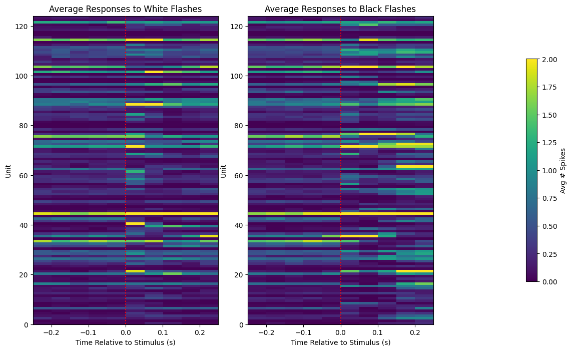
def get_zscore_mat(spike_matrix, stimulus_onset_idx):
    """
    Inputs:
    The 3D spike matrix with dimensions, Unit * Trial * Time, where values are the # of spikes in each bin
    The index of the time dimension when we expect the stimulus to be shown

    Outputs:
    A 2D matrix with dimensions Unit * Time, where values are the trial-averaged z-scores between the pre-stimulus (baseline) and post-stimulus (evoked) time periods
    Z-score for each bin is defined as the (bin value - baseline mean) / baseline standard deviation
    """

    baseline_rates = np.mean(spike_matrix[:,:,:stimulus_onset_idx], axis=2)
    baseline_stds = np.std(spike_matrix[:,:,:stimulus_onset_idx], axis=2)

    mean_baseline_rate = np.expand_dims(np.mean(baseline_rates, axis=1), 1)
    mean_baseline_stds = np.expand_dims(np.mean(baseline_stds, axis=1), 1) + 0.1 # to prevent division by 0

    zscores = (np.mean(spike_matrix, axis=1) - mean_baseline_rate) / mean_baseline_stds
    return zscores

white_flash_zscores = get_zscore_mat(white_flash_responses, stimulus_onset_idx)
black_flash_zscores = get_zscore_mat(black_flash_responses, stimulus_onset_idx)

print(white_flash_zscores.shape)
print(black_flash_zscores.shape)
(124, 10)
(124, 10)
fig, axes = plt.subplots(1, 3, figsize=(13,8), gridspec_kw={"width_ratios":[1,1,0.4]})
vmax=2
axes[0].imshow(white_flash_zscores, vmax=vmax, extent=[bin_edges[0], bin_edges[-1], 0, len(units_spike_times)], aspect="auto")
axes[0].vlines(0, white_flash_zscores.shape[0], 0, colors="r", ls=":")
axes[0].set_title("Average Z-Scores for White Flashes")
axes[0].set_xlabel("Time Relative to Stimulus (s)")
axes[0].set_ylabel("Unit")

img = axes[1].imshow(black_flash_zscores, vmax=vmax, extent=[bin_edges[0], bin_edges[-1], 0, len(units_spike_times)], aspect="auto")
axes[1].vlines(0, black_flash_zscores.shape[0], 0, colors="r", ls=":")
axes[1].set_title("Average Z-Scores for Black Flashes")
axes[1].set_xlabel("Time Relative to Stimulus (s)")
axes[1].set_ylabel("Unit")

cbar = fig.colorbar(img, ax=axes[2])
axes[2].set_visible(False)
cbar.set_label("Avg Z-Score")
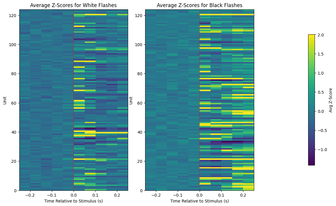
Selecting Most Responsive Units#
Of the units whose z-scores are shown above, the most responsive ones are selected and plotted if their maximum z-score is greater than 2. It can be seen that there are many more units with high z-scores for black flashes. This is more evidence that units are more responsive to the black flash stimulus rather than white flashes.
# pick top 10 most responsive units
white_max_zscores = np.max(white_flash_zscores[:,stimulus_onset_idx:], axis=1)
top_white_units = np.nonzero(white_max_zscores > 2)[0]
top_white_zscores = white_flash_zscores[top_white_units]

black_max_zscores = np.max(black_flash_zscores[:,stimulus_onset_idx:], axis=1)
top_black_units = np.nonzero(black_max_zscores > 2)[0]
top_black_zscores = black_flash_zscores[top_black_units]
fig, axes = plt.subplots(1, 3, figsize=(13,4), gridspec_kw={"width_ratios":[1,1,0.4]})

axes[0].imshow(top_white_zscores, vmax=3, extent=[bin_edges[0], bin_edges[-1], 0, len(top_white_units)], aspect=0.02)
axes[0].vlines(0, top_white_zscores.shape[0], 0, colors="r", ls=":")
axes[0].set_title("Most Responsive Units to White Flashes")
axes[0].set_xlabel("Time Relative to Stimulus (s)")
axes[0].set_ylabel("Selected Unit")
axes[1].imshow(top_black_zscores, vmax=3, extent=[bin_edges[0], bin_edges[-1], 0, len(top_black_units)], aspect=0.02)
axes[1].vlines(0, top_black_zscores.shape[0], 0, colors="r", ls=":")
axes[1].set_title("Most Responsive Units to Black Flashes")
axes[1].set_xlabel("Time Relative to Stimulus (s)")
axes[1].set_ylabel("Selected Unit")

cbar = fig.colorbar(img, ax=axes[2])
axes[2].set_visible(False)
cbar.set_label("Avg # Spikes")
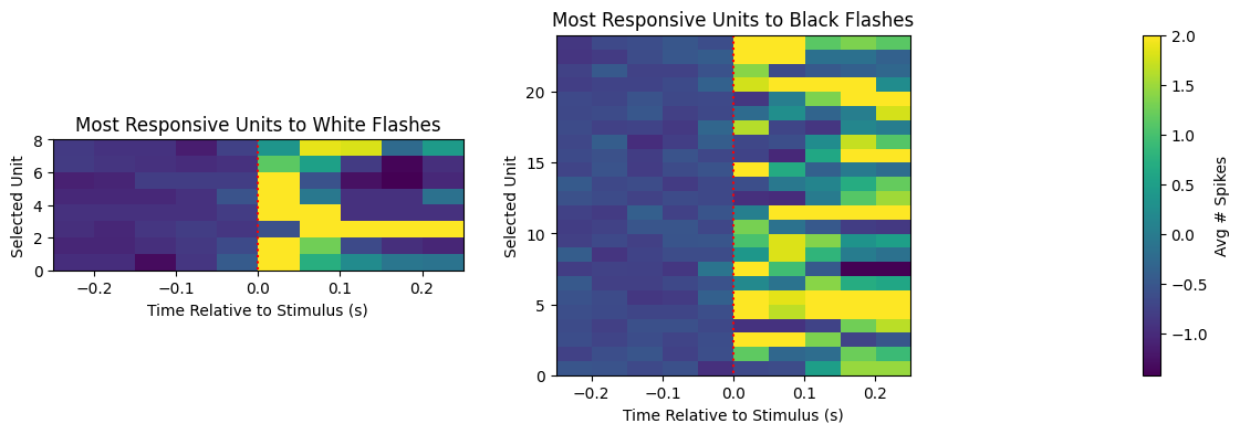
Comparing Z-Scores with GLM Filters#
As we’ve seen, both the trained GLM filter and the response Z-scores can give an interpretation of unit responsiveness. Below, the most responsive units from estimations of the strongest Z-Scores and the best fitting GLMs are plotted and compared.
It can be noticed that the filters may be negative. Recall that when the spiking probability is predicted by the GLM, the trained filter is convolved over the input stimulus, and then added to by a trained constant that represents the baseline firing rate. This means a negative filter indicates that a recent stimulus will decrease the predicted firing rate and a positive filter will increase predicted firing rate, relative to the trained constant’s baseline firing rate.
Another thing that might be noticed is that the filters sometimes appear to be a mirror image the stimulus evoked spiking over time. This is expected. Since the filters are convolved over the stimulus with each time point being negative, the resulting shape would resemble something like the forward response shown in the spiking plots.
It is important to note that because we are selected units that are apparently the most responsive, these filters and spike counts will be the clearest and most meaningful examples. Many of the other filters may just represent noise or be much harder to interpret.
print("Units most responsive to white flashes:", np.sort(top_white_units))
print("Units most responsive to black flashes:", np.sort(top_black_units))
print("Units that produced best fitting GLMs for white flashes:", np.nonzero(white_best_fits)[0])
print("Units that produced best fitting GLMs for black flashes:", np.nonzero(black_best_fits)[0])
Units most responsive to white flashes: [  3  55  62  67  83  84  86 102]
Units most responsive to black flashes: [  3  26  42  47  51  53  55  58  60  67  70  71  77  78  79  85  88  96
 102 108 109 115 119 121]
Units that produced best fitting GLMs for white flashes: [84]
Units that produced best fitting GLMs for black flashes: [  3  13  14  20  47  51  52  53  55  58  60  62  69  70  77  79  83  85
  86  88  95  96 102 108 109 119 120 121]
units_of_interest = reduce(np.union1d, (top_white_units, top_black_units, np.nonzero(white_best_fits)[0], np.nonzero(black_best_fits)[0]))

fig, axes = plt.subplots(len(units_of_interest), 4, figsize=(25, 2*len(units_of_interest)))
for i, unit_id in enumerate(units_of_interest):
    spikes_binned, constant, white_filter, black_filter = training_outputs[unit_id]
    mean_white_response = np.mean(white_flash_responses[unit_id], axis=0)
    mean_black_response = np.mean(black_flash_responses[unit_id], axis=0)

    axes[i][0].plot(filter_time_bins[1:], white_filter, color="silver")
    axes[i][1].plot(bin_edges[stimulus_onset_idx:-1], mean_white_response[stimulus_onset_idx:], color="silver")
    axes[i][2].plot(filter_time_bins[1:], black_filter, color="black")
    axes[i][3].plot(bin_edges[stimulus_onset_idx:-1], mean_black_response[stimulus_onset_idx:], color="black")

# give axis labels to first and last plots
for ax_x, ax_y in ((0,0), (0,1), (0,2), (0,3), (-1,0), (-1,1), (-1,2), (-1,3)):
    axes[ax_x][ax_y].set_xlabel("Time Relative to Stimulus")

for ax_x, ax_y in ((0,0), (0,2), (-1,0), (-1,2)):
    axes[ax_x][ax_y].set_ylabel("Unitless")

for ax_x, ax_y in ((0,1), (0,3), (-1,1), (-1,3)):
    axes[ax_x][ax_y].set_ylabel("# Spikes")

axes[0][0].set_title("Trained Filter for White Flashes")
axes[0][1].set_title("Average White Flash Response")
axes[0][2].set_title("Trained Filter for Black Flashes")
axes[0][3].set_title("Average Black Flash Response")
fig.suptitle("Comparison of Selected Units' Filters and Responses", y=0.999)
fig.tight_layout()