Visualizing Unit Spikes

In our files, the data contains a spike train array for each putative neuron. These are arrays of timestamps that a neuron spikes. Since neurons spike different numbers of times and during different times, it would be difficult to analyze many neurons together with the data in this form. One way to solve this is to make a 3-Dimensional spike matrix. This is a 3D array with the dimensions neurons, time, and trials. The spike matrix consists of time bins which contain the count of spikes at each time, for each neuron, and for each trial. The spike matrix can be slices or averaged to produce useful 2D plots, or can be plugged in to more complex analysis. One application of this can be seen in Statistically Testing Spike Responses to Stimulus.

Environment Setup

⚠️Note: If running on a new environment, run this cell once and then restart the kernel⚠️

try:
    from databook_utils.dandi_utils import dandi_download_open
except:
    !git clone https://github.com/AllenInstitute/openscope_databook.git
    %cd openscope_databook
    %pip install -e .

import matplotlib as mpl
import matplotlib.pyplot as plt
import numpy as np

from scipy.io import savemat

%matplotlib inline

Downloading Ecephys File

Change the values below to download the file you’re interested in. In this example, we the Units table of an Ecephys file from The Allen Institute’s Visual Coding - Neuropixels dataset, so you’ll have to choose one with the same kind of data. Set dandiset_id and dandi_filepath to correspond to the dandiset id and filepath of the file you want. If you’re accessing an embargoed dataset, set dandi_api_key to your DANDI API key.

dandiset_id = "000021"
dandi_filepath = "sub-717038285/sub-717038285_ses-732592105.nwb"
download_loc = "."
dandi_api_key = None

io = dandi_download_open(dandiset_id, dandi_filepath, download_loc, dandi_api_key=dandi_api_key)
nwb = io.read()

PATH                            SIZE   DONE            DONE% CHECKSUM STATUS          MESSAGE
sub-717038285_ses-732592105.nwb 2.9 GB 2.9 GB           100%    ok    done                   
Summary:                        2.9 GB 2.9 GB                         1 done                 
                                       100.00%                                               
Downloaded file to ./sub-717038285_ses-732592105.nwb
Opening file

c:\Users\carter.peene\AppData\Local\Programs\Python\Python39\lib\site-packages\hdmf\spec\namespace.py:531: UserWarning: Ignoring cached namespace 'hdmf-common' version 1.1.3 because version 1.5.1 is already loaded.
  warn("Ignoring cached namespace '%s' version %s because version %s is already loaded."
c:\Users\carter.peene\AppData\Local\Programs\Python\Python39\lib\site-packages\hdmf\spec\namespace.py:531: UserWarning: Ignoring cached namespace 'core' version 2.2.2 because version 2.5.0 is already loaded.
  warn("Ignoring cached namespace '%s' version %s because version %s is already loaded."

Getting Units Data and Stimulus Data

Below, the Units table is retrieved from the file. It contains many metrics for every putative neuronal unit, printed below. For the analysis in this notebook, we are only interested in the spike_times attribute. This is an array of timestamps at which a spike is measured for that unit.

units = nwb.units
units.colnames

('velocity_below',
 'amplitude_cutoff',
 'repolarization_slope',
 'snr',
 'firing_rate',
 'waveform_duration',
 'presence_ratio',
 'isi_violations',
 'cumulative_drift',
 'spread',
 'max_drift',
 'PT_ratio',
 'nn_hit_rate',
 'quality',
 'recovery_slope',
 'velocity_above',
 'isolation_distance',
 'l_ratio',
 'peak_channel_id',
 'd_prime',
 'cluster_id',
 'amplitude',
 'waveform_halfwidth',
 'local_index',
 'silhouette_score',
 'nn_miss_rate',
 'spike_times',
 'spike_amplitudes',
 'waveform_mean')

units[:10]

	velocity_below	amplitude_cutoff	repolarization_slope	snr	firing_rate	waveform_duration	presence_ratio	isi_violations	cumulative_drift	spread	...	d_prime	cluster_id	amplitude	waveform_halfwidth	local_index	silhouette_score	nn_miss_rate	spike_times	spike_amplitudes	waveform_mean
id
915957951	-0.343384	0.000886	0.880810	4.800479	2.035908	0.686767	0.98	0.000000	53.49	50.0	...	6.214486	323	234.454545	0.137353	314	0.229600	0.000102	[58.4338983925338, 68.84436108646727, 69.12766...	[0.00035119779048895465, 0.0003151291869021440...	[[0.0, 0.2250300000000216, 2.9977350000000555,...
915957946	0.000000	0.000217	0.400703	3.429461	5.738931	0.714238	0.99	0.009670	123.55	50.0	...	6.316538	322	138.920730	0.151089	313	0.158374	0.000906	[1.021669806312146, 1.1772369117243047, 2.5084...	[0.00016757406732947436, 0.0001720397921770987...	[[0.0, -3.2106749999999806, 3.150420000000011,...
915957691	-1.103733	0.014154	0.426480	1.919786	2.008079	0.796650	0.99	2.705249	290.95	100.0	...	3.662792	275	147.761055	0.206030	268	0.158752	0.001013	[0.6530354333202749, 3.2586094484803794, 3.264...	[7.60907503923193e-05, 7.957109416173626e-05, ...	[[0.0, -11.971440000000083, -12.44139000000006...
915957685	-0.956569	0.000230	0.842665	4.186323	4.709665	0.837856	0.99	0.005385	53.80	90.0	...	5.161656	274	260.690625	0.192295	267	0.234811	0.000138	[1.2490037807948806, 1.2540371283237506, 1.831...	[0.000266164371359917, 0.0002605838430779542, ...	[[0.0, -5.997810000000001, 5.6064450000000186,...
915956513	0.343384	0.500000	0.562422	3.457604	2.181748	0.645561	0.99	0.209098	139.54	60.0	...	2.918675	43	221.177190	0.247236	43	0.057446	0.003356	[3.2777428357755536, 11.522366088064498, 12.26...	[0.000144906487588058, 0.00010868803407731714,...	[[0.0, 0.0228149999999836, 2.534804999999988, ...
915956508	1.030151	0.000004	0.958932	5.408729	6.252715	0.494472	0.99	0.001018	30.54	50.0	...	6.895246	42	322.610340	0.192295	42	0.212086	0.002584	[14.719841772563301, 22.41733014843588, 30.700...	[0.0002151604191262871, 0.00020362049040077184...	[[0.0, 7.416434999999929, 3.2403149999999847, ...
915956502	-1.030151	0.001222	0.513393	3.237491	16.870943	0.563149	0.99	0.031472	83.51	40.0	...	4.833891	41	187.746780	0.206030	41	0.218050	0.001938	[1.4603043767253872, 1.4698044035182873, 1.481...	[0.00015597232901272, 0.0002357881951492309, 0...	[[0.0, -1.0518299999999812, -1.572479999999974...
915957820	0.423506	0.500000	0.451907	3.245378	0.008816	0.192295	0.26	0.000000	0.00	90.0	...	2.035774	300	113.818916	0.109883	292	NaN	0.000000	[461.1188340837827, 4209.908773452706, 4513.18...	[6.916100951089473e-05, 0.00010573897883329469...	[[0.0, -7.005903614457829, -4.6729518072289125...
915957814	-0.686767	0.219911	0.377458	2.882758	2.044300	0.274707	0.91	0.152423	211.72	20.0	...	6.940011	299	90.401025	0.109883	291	0.063454	0.000170	[403.78390571557065, 540.1631903457029, 1001.0...	[8.160101108265708e-05, 8.231111987309405e-05,...	[[0.0, -2.198040000000006, 8.860604999999943, ...
915956679	0.240369	0.013547	0.198606	0.862630	0.497001	0.412060	0.99	56.734425	787.79	170.0	...	4.532952	73	61.062105	0.260972	73	NaN	0.000100	[32.79502608329068, 32.81382613631242, 32.8917...	[7.08162454791397e-05, 5.720387439876228e-05, ...	[[0.0, -0.5660849999999442, 1.869854999999987,...

10 rows × 29 columns

units_spike_times = units["spike_times"]
print(units_spike_times.shape)

(3076,)

Selecting Stimulus Times

Different types of stimulus require different kinds of inclusion criteria. Since the available stimulus tables vary significantly depending which NWB file and which experimental session you’re analyzing, you’ll may have to adjust some values below for your analysis. First, select which stimulus table you want by changing the key used below in nwb.intervals. The list of stimulus table names is printed below to inform this choice. Additionally, you’ll have to modify the function stim_select to select the stimulus times you want to use. In this example, the stimulus type is the presentation of Gabor patches, and the stimulus times are chosen where a Gabor patch is shown at x and y coordinates 40, 40.

stimulus_names = list(nwb.intervals.keys())
print(stimulus_names)

['drifting_gratings_presentations', 'flashes_presentations', 'gabors_presentations', 'invalid_times', 'natural_movie_one_presentations', 'natural_movie_three_presentations', 'natural_scenes_presentations', 'spontaneous_presentations', 'static_gratings_presentations']

stim_table = nwb.intervals["gabors_presentations"]
print(stim_table.colnames)
stim_table[:10]

('start_time', 'stop_time', 'stimulus_name', 'stimulus_block', 'temporal_frequency', 'x_position', 'y_position', 'color', 'mask', 'opacity', 'phase', 'size', 'units', 'stimulus_index', 'orientation', 'spatial_frequency', 'contrast', 'tags', 'timeseries')

	start_time	stop_time	stimulus_name	stimulus_block	temporal_frequency	x_position	y_position	color	mask	opacity	phase	size	units	stimulus_index	orientation	spatial_frequency	contrast	tags	timeseries
id
0	81.645874	81.879397	gabors	0.0	4.0	-30.0	-20.0	[1.0, 1.0, 1.0]	circle	1.0	[3644.93333333, 3644.93333333]	[20.0, 20.0]	deg	0.0	45.0	0.08	0.8	[stimulus_time_interval]	[(1, 1, timestamps pynwb.base.TimeSeries at 0x...
1	81.879397	82.129600	gabors	0.0	4.0	20.0	-10.0	[1.0, 1.0, 1.0]	circle	1.0	[3644.93333333, 3644.93333333]	[20.0, 20.0]	deg	0.0	90.0	0.08	0.8	[stimulus_time_interval]	[(2, 1, timestamps pynwb.base.TimeSeries at 0x...
2	82.129600	82.379803	gabors	0.0	4.0	40.0	30.0	[1.0, 1.0, 1.0]	circle	1.0	[3644.93333333, 3644.93333333]	[20.0, 20.0]	deg	0.0	90.0	0.08	0.8	[stimulus_time_interval]	[(3, 1, timestamps pynwb.base.TimeSeries at 0x...
3	82.379803	82.630006	gabors	0.0	4.0	40.0	-40.0	[1.0, 1.0, 1.0]	circle	1.0	[3644.93333333, 3644.93333333]	[20.0, 20.0]	deg	0.0	45.0	0.08	0.8	[stimulus_time_interval]	[(4, 1, timestamps pynwb.base.TimeSeries at 0x...
4	82.630006	82.880215	gabors	0.0	4.0	-30.0	10.0	[1.0, 1.0, 1.0]	circle	1.0	[3644.93333333, 3644.93333333]	[20.0, 20.0]	deg	0.0	45.0	0.08	0.8	[stimulus_time_interval]	[(5, 1, timestamps pynwb.base.TimeSeries at 0x...
5	82.880215	83.130425	gabors	0.0	4.0	30.0	10.0	[1.0, 1.0, 1.0]	circle	1.0	[3644.93333333, 3644.93333333]	[20.0, 20.0]	deg	0.0	45.0	0.08	0.8	[stimulus_time_interval]	[(6, 1, timestamps pynwb.base.TimeSeries at 0x...
6	83.130425	83.380635	gabors	0.0	4.0	-40.0	-10.0	[1.0, 1.0, 1.0]	circle	1.0	[3644.93333333, 3644.93333333]	[20.0, 20.0]	deg	0.0	0.0	0.08	0.8	[stimulus_time_interval]	[(7, 1, timestamps pynwb.base.TimeSeries at 0x...
7	83.380635	83.630844	gabors	0.0	4.0	-10.0	20.0	[1.0, 1.0, 1.0]	circle	1.0	[3644.93333333, 3644.93333333]	[20.0, 20.0]	deg	0.0	0.0	0.08	0.8	[stimulus_time_interval]	[(8, 1, timestamps pynwb.base.TimeSeries at 0x...
8	83.630844	83.881050	gabors	0.0	4.0	10.0	30.0	[1.0, 1.0, 1.0]	circle	1.0	[3644.93333333, 3644.93333333]	[20.0, 20.0]	deg	0.0	90.0	0.08	0.8	[stimulus_time_interval]	[(9, 1, timestamps pynwb.base.TimeSeries at 0x...
9	83.881050	84.131255	gabors	0.0	4.0	30.0	-20.0	[1.0, 1.0, 1.0]	circle	1.0	[3644.93333333, 3644.93333333]	[20.0, 20.0]	deg	0.0	90.0	0.08	0.8	[stimulus_time_interval]	[(10, 1, timestamps pynwb.base.TimeSeries at 0...

### select start times from table that fit certain criteria here

stim_select = lambda row: True
stim_select = lambda row: float(row.x_position) == 40 and float(row.y_position) == 40
stim_times = [float(stim_table[i].start_time) for i in range(len(stim_table)) if stim_select(stim_table[i])]
print(len(stim_times))

45

Getting Unit Spike Response Counts

With stimulus times selected for each trial, we can generate a spike matrix to perform our analysis on. The spike matrix will have dimensions Units, Time, and Trials. You may set time_resolution to be the duration, in seconds, of each time bin in the matrix. Additionally, window_start_time, and window_end_time can be set to the time, in seconds, relative to the onset of the stimulus at time 0. Finally, the stimulus matrix will also be averaged across trials to get the average spike counts over time for each unit, called mean_spike_counts.

# bin size for counting spikes
time_resolution = 0.005

# start and end times (relative to the stimulus at 0 seconds) that we want to examine and align spikes to
window_start_time = -0.25
window_end_time = 0.75

# time bins used
n_bins = int((window_end_time - window_start_time) / time_resolution)
bin_edges = np.linspace(window_start_time, window_end_time, n_bins, endpoint=True)

# useful throughout analysis
n_units = len(units_spike_times)
n_trials = len(stim_times)

# calculate baseline and stimulus interval indices for use later
stimulus_onset_idx = int(-bin_edges[0] / time_resolution)

# 3D spike matrix to be populated with spike counts
spike_matrix = np.zeros((n_units, len(bin_edges), n_trials))

# populate 3D spike matrix for each unit for each stimulus trial by counting spikes into bins
for unit_idx in range(n_units):
    spike_times = units_spike_times[unit_idx]

    for stim_idx, stim_time in enumerate(stim_times):
        # get spike times that fall within the bin's time range relative to the stim time        
        first_bin_time = stim_time + bin_edges[0]
        last_bin_time = stim_time + bin_edges[-1]
        first_spike_in_range, last_spike_in_range = np.searchsorted(spike_times, [first_bin_time, last_bin_time])
        spike_times_in_range = spike_times[first_spike_in_range:last_spike_in_range]

        # convert spike times into relative time bin indices
        bin_indices = ((spike_times_in_range - (first_bin_time)) / time_resolution).astype(int)
        
        # mark that there is a spike at these bin times for this unit on this stim trial
        for bin_idx in bin_indices:
            spike_matrix[unit_idx, bin_idx, stim_idx] += 1

spike_matrix.shape

(3076, 200, 45)

Spike Plots From Spike Matrix

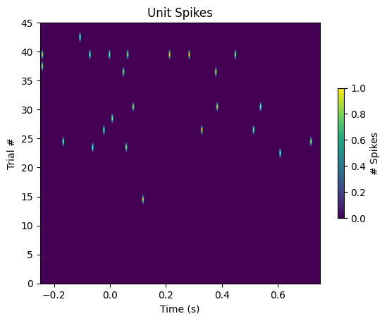
To demonstrate visually how it can be used, the plots below show different slices of the spike matrix. The first plot, Unit Spikes Across Trials shows the spiking behavior of one Unit across all trials. Set unit below to change which unit you’d like be shown. Following this is the Unitwise Spike Plot, which shows the spikes of all Units during the time window of one trial. Finally, the Average Unitwise Spike Plot shows the spikes of all units averaged across all trials. By themselves, these plots don’t tell much. Useful versions of similar plots are depicted in notebooks such as Identifying Optotagged Units, and Statistically Testing Spike Responses to Stimulus

Unit Spikes Across Trials

unit = 0

fig, ax = plt.subplots()

ax.set_title("Unit Spikes")
ax.set_xlabel("Time (s)")
ax.set_ylabel("Trial #")

img = ax.imshow(spike_matrix[unit,:,:].transpose(), extent=[window_start_time,window_end_time,0,n_trials], aspect="auto")
cbar = fig.colorbar(img, shrink=0.5)
cbar.set_label("# Spikes")

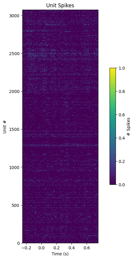
Unitwise Spike Plot

trial = 0

fig, ax = plt.subplots(figsize=(10,10))

ax.set_title("Unit Spikes")
ax.set_xlabel("Time (s)")
ax.set_ylabel("Unit #")

img = ax.imshow(spike_matrix[:,:,trial], extent=[window_start_time,window_end_time,0,n_units], aspect=0.001, vmin=0, vmax=1)
cbar = fig.colorbar(img, shrink=0.5)
cbar.set_label("# Spikes")

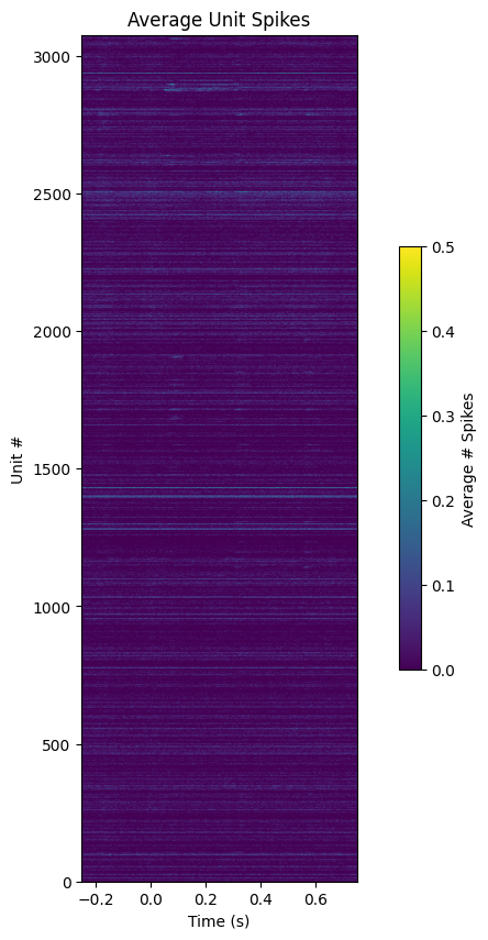
Average Unitwise Spike Plot

fig, ax = plt.subplots(figsize=(10,10))

ax.set_title("Average Unit Spikes")
ax.set_xlabel("Time (s)")
ax.set_ylabel("Unit #")

img = ax.imshow(np.average(spike_matrix, axis=2), extent=[window_start_time,window_end_time,0,n_units], aspect=0.001, vmin=0, vmax=0.5)
cbar = fig.colorbar(img, shrink=0.5)
cbar.set_label("Average # Spikes")

Saving Spike Matrix

The spike matrix can be saved/exported for use in other programs using several methods. Below, numpy’s save method is used to save the matrix in the npy format for use in other Python programs. Scipy’s savemat function saves the matrix in a format usable for Matlab.

np.save("spike_matrix.npy", spike_matrix)

savemat("spike_matrix.mat", dict(spike_matrix=spike_matrix))