Pulse Average (PA) plot

The purpose of the pulse averaging (PA) plot is to identify synaptic connections by pooling (via time alignment) and averaging the responses within and across sweeps to pulses (intended to produce action potentials) on a single headstage. It repeats this process for all headstages with pulses (action potentials).

Although the stimulus set will contain Pulse Train epochs in most cases, the pulse extraction algorithm works with all epoch types and special measurement modes like Distributed DAQ (dDAQ) or Optimized overlap distributed DAQ (oodDAQ).

The dDAQ slider from the Settings tab is respected as is the Channel Selection.

For instructional purposes, assume pulse train acquisition on four different headstages with oodDAQ (to distribute the pulses in time, across headstages). The PA plot shows AD data from each headstage and will have 16 (4 rows x 4 columns) PA sets (either in 16 plots on a single graph or 16 individual graphs; user-defined).

The diagonal entries hold the extracted single pulses for each headstage. In the other rows of each column are the regions plotted which are extracted from the other headstages at the same time coordinates as the diagonal pulses. So each row shows different regions from the same headstages, and each column shows the same region but from different headstages.

The following two figures, Trace plot and Image plot, were created with multiple sweeps overlayed, see Overlay Sweeps, and time alignment and zeroing turned on.

Trace plot

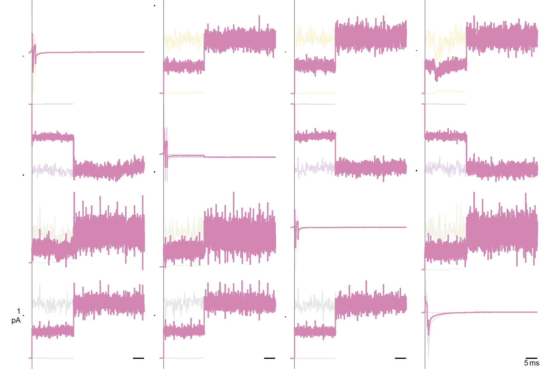
Trace plot

The trace plot displays data in each PA set as voltage or current time-series. Scale bars, shown in black, are provided for each y axes and for each column’s shared x (time) axes. PA trace colors match databrowser trace colors and encode the headstage, see also Relevant Colors.

Image plot

   

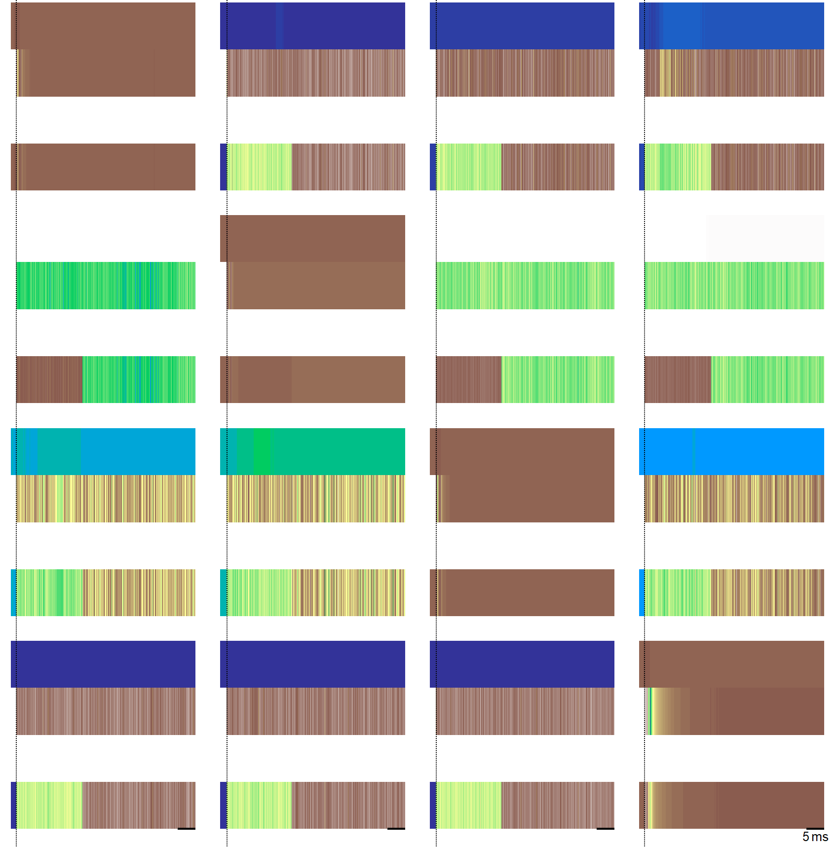
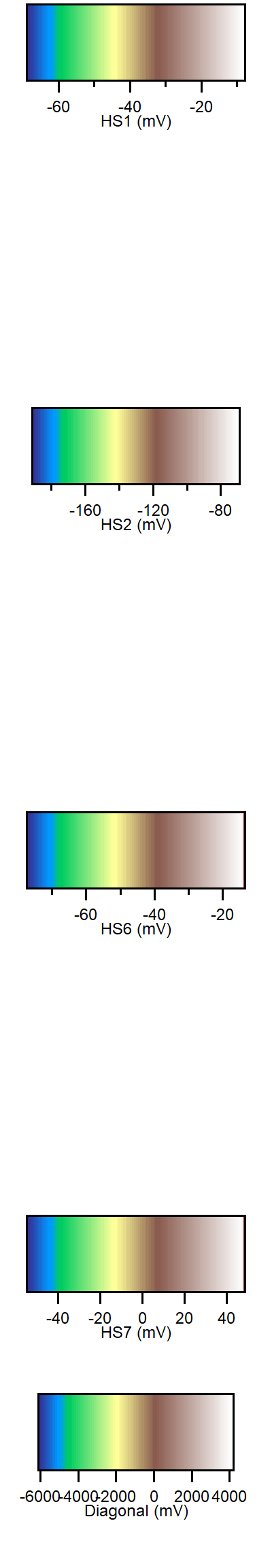
The image graph supplements the trace plot Trace plot. It renders more quickly than the trace plot, especially with many (overlayed) sweeps. Each (horizontal) line of the image plot corresponds to a pulse (unique time-series) and encodes the voltage or current in color (user-defined color mapping). Deconvolution and average lines (extra wide) are at the bottom of each set image. Image-space is left blank when data is not shown. The image is filled from top to bottom where the interleaving between pulses and sweeps depends on the Sort Order.

Sort Order

The following tables visualizes the display of one image set with two sweeps overlayed and three pulses using different Sort Order settings. The ordering is always ascending and from top to bottom. Due to implementation details the Sweep sort order allows much faster incremental updates (only relevant during data acqisition).

Comparing different sort orders

Sweep	Pulse
Pulse 0, Sweep 0	Pulse 0, Sweep 0
Pulse 1, Sweep 0	Pulse 0, Sweep 1
Pulse 2, Sweep 0	Pulse 1, Sweep 1
Pulse 0, Sweep 1	Pulse 1, Sweep 0
Pulse 1, Sweep 1	Pulse 2, Sweep 1
Pulse 2, Sweep 1	Pulse 2, Sweep 0
Average	Average
Deconvolution	Deconvolution

Time Alignment

Time alignment removes the pulse to pulse jitter in pulse evoked event (action potential) timing.

The algorithm is as follows:

• Get the feature position featurePos (wave maximum) for all pulses which belong to the same set. Store these feature positions using their sweep number and pulse index as key.

• Now shift all pulses in all sets from the same region by -featurePos where featurePos is used from the same sweep and pulse index.

Operation order

Data operations occur in the following (fixed) order:

• Gather pulses

• Pulse sorting

• Failed pulse search

• Zeroing

• Time alignment

• Averaging

PA plot settings

The following sections describe PA settings. Settings are configured on the data browser PA settings tab (shown below).

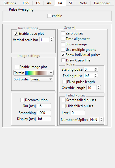
Settings for the pulse average plot

Pulse Averaging

• enable: Toggle the display of the PA image/trace plots.

  To adjust multiple settings at-a-time, disable the PA plot, adjust settings, and re-enable.

Image settings

• Enable image plot: Toggle the display of the Image plot

• Draw X zero line: Draws vertical line at X == 0 in each column. Requires time alignment

  (see below). Facilitates measurement of event latency.

• Popup Menu: Color scheme for image plots

• Sort order: Sort order of the displayed pulses. For Sweep the pulses are first ordered by sweep number and then by pulse index. For Pulse it is first pulse index and then sweep number. See also Sort Order.

Trace settings

• Enable trace plot: Toggle the display of the Trace plot.

• Vertical scale bar: Size of the vertical scale bar in y-axis units

Deconvolution

• Deconvolution: Enables deconvolution [4] of the average pulse. Deconvolution trace is displayed with the average trace in the trace plot and immediately above the average line in the image plot.

• Tau [ms]: Time constant [5]

• Smoothing: Smoothing parameter, use 1 to disable smoothing

• Display [ms]: Time range of the average pulse used for the deconvolution, use inf to use the full range

General

• Zero pulse: Toggle Pulse Zeroing. Zeroing is carried out by differentiation, followed by the integration of each pulse.

• Time alignment: Toggle time alignment of pulses from one column. See Time Alignment for an in-depth explanation.

• Show average: Toggle average pulse display. For the image plot, the average is the bottom-most row. Failed pulses (see below) are not included in the average.

• Use multiple graphs: Creates a panel for each PA set. Normally, multiple PA sets are distributed onto a single panel.

• Show individual pulses: Enables the display of individual pulses. Turning that off can increase the display update performance. The average and deconvolution are still shown if enabled.

Pulses

Select a subset of the pulses from a train of pulses (contained within a sweep).

• Starting pulse: First pulse index to display, 0-based.

• Ending pulse: Last pulse index to display, use inf to use the last pulse.

• Fixed pulse length: Choose the calculation method of the pulse lengths. When unchecked the pulse length is calculated as the average pulse length from the extracted pulses. When checked the Override length is used.

• Override length: Pulse length to use when no length can be calculated [6] or when Fixed pulse length is checked

Failed Pulses

Pulse responses may be filtered by their amplitude.

• Search failed pulses: Toggle the failed pulse search

• Hide failed pulses: When a pulse failed, hide instead of highlight.

• Level: Level in y-data units to search for failed pulses. Every pulse not reaching that level is considered failing. As mentioned in Operation order that search is done before zeroing.

• Number of Spikes: Number of required spikes for each pulse. Use NaN for accepting any non-zero spike count as passing.

[4]

See doi:10.1152/jn.00942.2007 for the implemented method

[5]

The following equation holds:

\[\tau \cdot \frac{dV}{dt} + V = f\]

[6]

Pulse length cannot be calculated when a sweep contains a single pulse or when the pulse length is variable, e.g., Poisson distribution from the Pulse Train stimulus epoch type.