The Sweep Formula Module¶

The Sweep Formula Module in MIES_Sweepformula.ipf is intended to be used from the SF tab in the BrowserSettingsPanel (BSP). It is useful for analyzing a range of sweeps using pre-defined functions. The backend parses a formula into a JSON logic like pattern which in turn is analyzed to return a wave for plotting.

Preprocessing¶

The entered code in the notebook is preprocessed. The preprocessor removes comments before testing the code for the ` vs ` operator after which it is passed to the formula parser. Comments start with a # character and end at the end of the current line.

Formula Parser¶

In order for a formula to get executed, it has to be analyzed. This assures that the correct order of calculations is used. The approach for solving this is using a token based state machine. We virtually insert one character at a time from left to right into the state machine. Usually, a character is collected into a buffer. At some special characters like a + sign, the state changes from collect to addition. If a state changes, a new evaluation group is created which is represented with a JSON object who’s (single) member is the operation. The member name is the operation and the value is an ordered array of the operands. To ensure that multiplication is executed before addition to get 1+2*3=7 and not 1+2*3=9 the states have a priority. Higher order states cause the operation order to switch. The old operation becomes part of the new operation. In this context, when the first array or function argument separator , is parsed on a level, it is treated as higher order operations because it creates a new array.

{
  "+": [
    1,
    {
      "*": [
        2,
        3
      ]
    }
  ]
}

Arrays start with a square bracket [ and end with a ]. Subsequent array elements are separated by a ,. In a series of arrays like [1, 2], [3, 4], [5, 6] the , after the ] is enforced by the parser. Arrays can be part of arrays. Since at its core very formula input is an array the series of arrays [1, 2], [3, 4], [5, 6] is implicitly a 2-dimensional array: [[1, 2], [3, 4], [5, 6]]. The same applies for simple inputs like 1, which is implicitly treated as 1-dimensional array: [1]. The input [[1]] instead is treated as 1x1 2-dimensional array. Arrays are special as also function arguments contain array elements. Therefore, an array can also simply be created by omitting the array brackets and only using element separators similar as in functions. The function max(1,2) is therefore treated the same as max([1,2]). Arrays can represent data and functions evaluate to arrays. Arrays can be of arbitrary size and can also be concatenated as in max(0,min(1,2),1).

{
  "max": [
    0,
    {
      "min": [
        1,
        2
      ]
    },
    1
  ]
}

A number can be entered as 1000, 1e3, or 10.0e2. It is always stored as a numeric value and not as string. The formula parser treats everything that is not parsable but matches alphanumeric characters (excluding operations) to a string as in a_string. White spaces are ignored throughout the formula which means that strings do not need to get enclosed by “. In fact, a “ is an disallowed character.

[
  1000,
  "a_string"
]

A function is defined as a string that is directly followed by an opening parenthesis. The parenthesis token causes to force a collect state until all parentheses are closed.

Everything that is collected in a buffer is sent back to the function via recursive execution. The formula parser only handles elements inside one recursion call that are linearly combinable like 1*2+3*4. If same operations follow each other, they are concatenated into the same array level as for 1+2+3+4.

{
  "+": [
    1,
    2,
    3,
    4
  ]
}

{
  "+": [
    {
      "*": [
        1,
        2
      ]
    },
    {
      "*": [
        3,
        4
      ]
    }
  ]
}

The formula is sent to a preparser that checks for the correct amount of brackets and converts multi-character operations to their multi-character UTF-8 representations like … to …. It should be noted that an operation consists of one UTF-8 character. Functions on the other hand can consist of an arbitrary length of alphanumeric characters. The corresponding function for the above operation is range().

Formula Executor¶

The formula executor receives a JSON id. It can only evaluate a specific structure of a formula which means for usual cases that it should start with an object that contains one operation. Operations are evaluated via recursive calls to the formula executor at different paths. This ensures that the formula is evaluated from the last element to the first element. The formula in the above example 1*2+3*4 is therefore parsed to

{
  "+": [
    {
      "*": [
        1,
        2
      ]
    },
    {
      "*": [
        3,
        4
      ]
    }
  ]
}

The execution follows these steps:

evaluate / to + operation, call +
called from + operation -> evaluate /+ array to array with two elements
evaluate /+/0 to * operation with an array argument with two elements 1, 2
called from * operation -> evaluate /+/0/* array to wave {1, 2}
* operation is applied to wave {1, 2}, returning wave {2}
insert wave {2} as first element of array from step 2
evaluate /+/1 to * operation with an array argument with two elements 3, 4
called from * operation -> evaluate /+/0/* array to wave {3, 4}
* operation is applied to wave {3, 4}, returning wave {12}
insert wave {12} as second element of array from step 2
+ operation is applied to wave {2, 12} returning wave {14}

At the time of an evaluation, the maximum depth of an array is four dimensions as Igor Pro supports only four dimensions. This implies that on recursive evaluation of multi dimensional arrays the sub arrays can be three dimensional at best.

Array Evaluation¶

The array evaluation supports numeric and text data. The interpretation of the JSON arrays as text data is preferred. This means that [“NaN”] returns a one element text wave {“NaN”}, whereas [1, “NaN”] returns a two element numeric wave {1, NaN}. If one element can not be parsed as string then it is assumed that the array contains numeric data. The JSON null element is only allowed for the topmost array as the parser inserts it for operation with no argument like e.g. select(). For sub arrays null elements [null] are invalid and result in an error.

If the topmost array is empty [] an empty numeric wave with zero size is returned. When checked in operation code the wave size should be checked before the wave type.

If the current array evaluated is of size one, then the wave note is transferred from the subArray to the current array. This is important for the case where the element of the current array is an JSON object, thus an operation, and the operation result is a single value with meta data in the wave.

Formula Executor Limitations¶

Mixed data types in arrays are not supported as this JSON property is hard to translate to Igor Pro data storage in waves.

Internal Data Layout¶

The data is stored internally in persistant wave reference waves in a data folder, e.g. root:MIES:HardwareDevices:Dev1:Databrowser:FormulaData:. The reason is that operation like data(…) should be able to return multiple independent sweep data waves. These can be returned through a wave reference wave. Each wave referenced contains numeric or text data. The formula executor works on the JSON data that was created by the formula parser only. This data is by definition either an object (operation), numeric or a textual. If an operation like data(…) returns sweep data of multiple sweeps in a persistent wave reference wave for the formula executor a single element text wave is created. This text wave encodes a marker and the path to the wave reference wave in the first element. The wave reference wave is resolved by wrapper functions when calling the formula executor, such that the formula executor works only with the data wave(s).

Wrapper functions are:

SF_GetArgument: retrieves an operation argument, returns a wave reference wave. If in the JSON from the parser the argument consists of ‘direct’ data like an array then it is automatically converted to a wave reference wave with one element that refers to the data wave.
SF_GetArgumentSingle: retrieves an operation argument expecting only a single data wave. Returns the data wave.
SF_GetArgumentTop: retrieves all operation arguments as an array, returns a wave reference wave.
SF_GetOutputForExecutor: Takes a wave reference wave as input and creates a single element text wave for returning further to the formula executor.
SF_GetOutputForExecutorSingle: Takes a data wave as input, creates a single element wave reference wave referring to the data wave and creates text wave for returning further to the formula executor.

The wrapper function imply that the formula executor is never called directly from operation code. Also directly parsing the JSON is not allowed in operation code because every argument could be another operation or multi dimensional array etc.

Debugging Formula Execution¶

By default only the currently used wave reference waves are persistent. For debugging the execution the SWEEPFORMULA_DEBUG define can be set: #define SWEEPFORMULA_DEBUG. When set all data waves and wave reference waves are stored persistently in the sweepformula working data folder that are created during the execution. The naming scheme is as follows: “source_pointOfCreation” with

source: typically the name of the operation or “ExecutorSubArrayEvaluation”

pointOfCreation:

output: wave reference wave output of operation
dataInput: data wave of direct data from JSON
refFromuserInput: wave reference wave automatically created to for data wave of direct data from JSON
return_argX_: data wave(s) returned by an operation, X counts the data waves aka index in the associated wave reference wave
argTop: prefix for the upper tags, added when data was parsed from the top level, used e.g. by integrate(1, 2)

The final wave name might be suffixed by a number guaranteeing unique wave names when multiple times the same operation was called.

Operations¶

In the context of the formula executor, different operations and functions are defined. Some of them are MIES specific, some of them are wrappers to Igor Pro operations or functions, some borrowed from other languages and there are also the simple, trivial operations. This section should give a list of the available operations and give a look into how they are meant to be used

The trivial operations are +, -, *, /. They are defined for all available dimensions and evaluate column based.

They can be used for evaluating

scalars with 1d waves as in 1 + [1, 2] = [1, 1] + [1, 2] = [2, 3]
1d waves with 1d waves as in [1, 2] + [3, 4] = [4, 6]
1d waves with 2d waves as in [1, 2] + [[3, 4], [5, 6]] = [[1 + 3, 2 + 5], [NaN + 4, NaN + 6]] = [[4, 7], [NaN, NaN]]
2d waves with 2d waves as in [[1, 2], [3, 4]] + [[5, 6], [7, 8]] = [[6, 8], [10, 12]]

The size in each dimension is expanded to match the maximum array size. The maximum array size is determined by the required maximum dimensions of the elements in the topmost array. An array element can be a number, a string, an array or an operation. A number or string a scalar. An sub array or operaton result is scalar if it returns a single element. The expansion is filled with for numeric waves with NaN or for textual waves with “”. In the special case of a scalar element, the value is expanded to the full size and dimensions of the expanded arrays size. This means that in our first example, 1 is scalar and is internally expanded to an array of size 2 because the second operand determines the maximum size of 2: 1 + [1, 2] == [1, 1] + [1, 2]. On the other hand in the third example above the first arrays size is expanded but not its value as it is not a scalar. The array size expansion and scalar elements expansion is applied recursively for more dimensions. Note that operations in array elements may return multi dimensional sub arrays that lead to an overall array expansion that is greater as the formula input suggests.

Statistical Operations¶

min and max¶

min and max return the minimum and maximum of an array. The operation takes 1 to N arguments. The input data must be 1d or 2d, numeric and have at least one data point. The operations work column based, such that for each column e.g. the maximum of all row values is determined. An 2d input array of size MxN is returned as 1d array of the size N. When called with a single argument the operation accepts multiple data waves. For this case the operation is applied on each input data wave independently and returns the same number of data waves. The returned data type is SF_DATATYPE_MIN or SF_DATATYPE_MAX. If input data type is SF_DATATYPE_SWEEP from the data operation the sweep meta data is transferred to the returned data waves. The default suggested x-axis values for the formula plotter are sweep numbers.

min([[1, 2],[3, 4]]) = [1, 2]

max(min([[1, 2],[3, 4]])) = [2]

min(2) == [2]

avg and mean¶

avg(array data[, string mode])

avg and mean are synonyms for the same operation. They calculate the arithmetic average $\frac{1}{n}\sum_i{x_i}$.

data: input data wave(s)

mode: optional parameter that defines in which direction the average is applied.

in default, applies the average over each input data wave. In this mode the operation returns the same number of waves as input waves were specified. Each output wave contains a single data point. If input data type is SF_DATATYPE_SWEEP from the data operation the sweep meta data is transferred to the returned data waves. The default suggested x-axis values for the formula plotter are sweep numbers.
over averages over all input data waves. In this mode the operation returns a single wave. NaN values in input waves are ignored in the average calculation. A trace generated from the returned wave will be shown as topmost trace in the default color for averaged data.

The returned data type is SF_DATATYPE_AVG.

avg([1, 2, 3]) == [2]

avg(data(ST, select(channels(AD), sweeps(), all)), over)

avg(data(ST, select()), in)

root mean square¶

rms calculates the root mean square $\sqrt{\frac{1}{n}\sum_i{x_i^2}}$ of a row if the wave is 1d. It calculates column based if the wave is 2d. The operation takes 1 to N arguments. The input data must be 1d or 2d, numeric and have at least one data point. The operations works column based, such that for each column e.g. the average of all row values is determined. An 2d input array of size MxN is returned as 1d array of the size N. When called with a single argument the operation accepts multiple data waves. For this case the operation is applied on each input data wave independently and returns the same number of data waves. The returned data type is SF_DATATYPE_RMS. If input data type is SF_DATATYPE_SWEEP from the data operation the sweep meta data is transferred to the returned data waves. The default suggested x-axis values for the formula plotter are sweep numbers.

rms(1, 2, 3) == [2.160246899469287]

rms([1, 2, 3],[2, 3, 4],[3, 4, 5]) == [2.160246899469287, 3.109126351029605, 4.08248290463863]

variance¶

variance calculates the variance of a row if the wave is 1d. It calculates column based if the wave is 2d. Note that compared to the Igor Pro function variance() the operation does not ignore NaN or Inf. The operation takes 1 to N arguments. The input data must be 1d or 2d, numeric and have at least one data point. The operations works column based, such that for each column e.g. the average of all row values is determined. An 2d input array of size MxN is returned as 1d array of the size N. When called with a single argument the operation accepts multiple data waves. For this case the operation is applied on each input data wave independently and returns the same number of data waves. The returned data type is SF_DATATYPE_VARIANCE. If input data type is SF_DATATYPE_SWEEP from the data operation the sweep meta data is transferred to the returned data waves. The default suggested x-axis values for the formula plotter are sweep numbers.

variance(1, 2, 4) == [2.33333]

variance([1, 2, 4],[2, 3, 2],[4, 2, 1]) == [2.33333, 0.33333, 2.33333]

stdev¶

stdev calculates the variance of a row if the wave is 1d. It calculates column based if the wave is 2d. The operation does not ignore NaN or Inf. The operation takes 1 to N arguments. The input data must be 1d or 2d, numeric and have at least one data point. The operations works column based, such that for each column e.g. the average of all row values is determined. An 2d input array of size MxN is returned as 1d array of the size N. When called with a single argument the operation accepts multiple data waves. For this case the operation is applied on each input data wave independently and returns the same number of data waves. The returned data type is SF_DATATYPE_STDEV. If input data type is SF_DATATYPE_SWEEP from the data operation the sweep meta data is transferred to the returned data waves. The default suggested x-axis values for the formula plotter are sweep numbers.

stdev(1, 2, 4) == [1.52753]

stdev([1, 2, 4],[2, 3, 2],[4, 2, 1]) == [1.52753, 0.57735, 1.52753]

Igor Pro Wrappers¶

area¶

Use area to calculate the area below a 1D array using trapezoidal integration.

area(array data[, variable zero])

The first argument is the data, the second argument specifies if the data is zeroed. Zeroing refers to an additional differentiation and integration of the data prior the area calculation. If the zero argument is set to 0 then zeroing is disabled. By default zeroing is enabled. If zeroing is enabled the input data must have at least 3 points. If zeroing is disabled the input data must have at least one point. The operation ignores NaN in the data. The operations works column based, such that for each column e.g. the area of all row values is determined. An 2d input array of size MxN is returned as 1d array of the size N. An 3d input array of size MxNxO is returned as 2d array of the size NxO. The operation accepts multiple data waves for the data argument. For this case the operation is applied on each input data wave independently and returns the same number of data waves. The returned data type is SF_DATATYPE_AREA. If input data type is SF_DATATYPE_SWEEP from the data operation the sweep meta data is transferred to the returned data waves. The default suggested x-axis values for the formula plotter are sweep numbers.

area([0, 1, 2, 3, 4], 0) == [8]

area([0, 1, 2, 3, 4], 1) == [4]

derivative¶

Use derivative to differentiate along rows for 1- and 2-dimensional data.

derivative(array data)

Central differences are used. The same amount of points as the input is returned. The input data must have at least one point. The operation ignores NaN in the data. The operation accepts multiple data waves for the data argument. For this case the operation is applied on each input data wave independently and returns the same number of data waves. The returned data type is SF_DATATYPE_DERIVATIVE.

derivative(1, 2, 4) == [1, 1.5, 2]

derivative([1, 2, 4],[2, 3, 2],[4, 2, 1]) == [1, 1, -2],[1.5, 0, -1.5],[2, -1, -1]

integrate¶

Use integrate to apply trapezoidal integration along rows. The operation returns the same number of points as the input wave(s).

integrate(array data)

Note that due to the end point problem it is not the counter-part of derivative. The input data must have at least one point. The operation ignores NaN in the data. The operation accepts multiple data waves for the data argument. For this case the operation is applied on each input data wave independently and returns the same number of data waves. The returned data type is SF_DATATYPE_INTEGRATE.

integrate(1, 2, 4) == [0, 1.5, 4.5]

integrate([1, 2, 4],[2, 3, 2],[4, 2, 1]) == [0, 0, 0],[1.5, 2.5, 3],[4.5, 5, 4.5]

butterworth¶

The operation butterworth applies a butterworth filter on the given data using FilterIIR from Igor Pro. The operation calculates along rows. It takes four arguments:

butterworth(array data, variable lowPassCutoffInHz, variable highPassCutoffInHz, variable order)

The first parameter data is intended to be used with the data() operation but can be an arbitrary numeric array. The parameters lowPassCutoffInHz and highPassCutoffInHz must be given in Hz. The maximum value for order is 100. The operation accepts multiple data waves for the data argument. For this case the operation is applied on each input data wave independently and returns the same number of data waves. The returned data type is SF_DATATYPE_BUTTERWORTH.

butterworth([0,1,0,1,0,1,0,1], 90E3, 100E3, 2) == [0, 0.863871, 0.235196, 0.692709, 0.359758, 0.60206, 0.425727, 0.554052]

xvalues and time¶

The function xvalues or time are synonyms for the same function. The function returns a wave containing the x-scaling of the input data.

xvalues(array data)

The output data wave has the same dimension as the input data. The x-scaling values are filled in the rows for all dimensions. The operation accepts multiple data waves for the data argument. For this case the operation is applied on each input data wave independently and returns the same number of data waves.

xvalues(10, 20, 30, 40, 50) == [0, 1, 2, 3, 4]

// The sweeps in this example were sampled at 250 kHz.
// For each data point in the sweep the time is returned.
time(data([0, 1000], channels(AD), sweeps())) == [0, 0.004, 0.008, 0.012, ...]

setscale¶

setscale sets a new wave scaling to an input wave. It accepts 2 to 5 arguments.

setscale(array data, string dim[, variable dimOffset[, variable dimDelta[, string unit]]])

data: input data wave
dim: dimension where the scale should be set, either d, x, y, z or t.
dimOffset: optional, the scale offset for the first data point. If not specified, 0 is used as default.
dimDelta: optional, the scale delta for the data point distance. If not specified, 1 is used as default.
unit: optional, the scale unit for the data points. If not specified, “” is used as default.

If d is used for dim, then in analogy to Igor Pros SetScale operation the dimOffset and dimDelta argument set the nominal minimum and nominal maximum data values of the wave.

If x, y, z or t is used for dim and dimDelta is 0 then the default dimDelta 1 is used.

The operation accepts multiple data waves for the data argument. For this case the operation is applied on each input data wave independently and returns the same number of data waves.

xvalues(setscale([0, 1, 2, 3, 4], x, 0, 0.2, firkin)) == [0, 0.2, 0.4, 0.6, 0.8]

channels¶

channels([str name]+) converts named channels from strings to numbers.

The function accepts an arbitrary amount of channel names like AD, DA or TTL with a combination of numbers AD1 or channel numbers alone like 2. The maximum allowed channel number is NUM_MAX_CHANNELS (16). For all channel types the channel numbers as given on the DAEphys panel are accepted. The operation returns a numeric array of [[channelType+], [channelNumber+]] that has as row dimension the number of the input strings. When called without argument all channel types / channel numbers are set by setting the returned value for type and number to NaN.

channels is intended to be used with the select() operation.

channels([AD0,AD1, DA0, DA1]) == [[0, 0, 1, 1], [0, 1, 0, 1]]

// Internally NaN is evaluated as joker for all channel types and all channel numbers
channels() == [[NaN], [NaN]]

sweeps¶

The operation sweeps return an 1d-array with the sweep numbers of all sweeps. The operation takes no arguments. If there are no sweeps a null wave is returned.

// For this example two sweeps were acquired
sweeps() == [0, 1]

cursors¶

The cursors operation returns the x-values of the named cursor(s).

cursors([A-J]+)

The cursors operation takes any number of arguments. If no argument is given it defaults to cursors(A, B). When cursors is used as argument for a range specification, e.g. for data two arguments for cursors should be used to have a compatible output. Valid cursor names are A-J. The operation returns a numeric 1d-wave containing the x-values of the named cursor(s). If a named cursor is not present, then NaN is returned as position.

cursors(A,B) vs A,B

cursors() vs A,B // same as above

cursors(B,A,D,J,I,G,G) // returns a 7 element array with the x-values of the named cursors

wave¶

The wave operation returns the content of the referenced wave.

wave(string pathToWave)

If no wave can be resolved at the given path a null wave is returned. The further handling depends how the operations receiving such null wave handles this special case. The formula plotter skips null waves.

wave(root:mywave)

text¶

The operation text converts the given numeric data to a text data.

text(array data)

This can be used to force, for example, a category plot. text requires numeric input data. The output data has the same dimension as the input data. The output precision for the text are 7 digits after the dot. The operation accepts multiple data waves for the data argument. For this case the operation is applied on each input data wave independently and returns the same number of data waves.

range(5) vs text(range(5))

data¶

The data operation is the core of the SweepFormula library. It returns sweep data from MIES. It can be called in two variants:

data(array range[, array selectData])

data(string epochShortName[, array selectData])

The range can be either supplied explicitly using [100, 300] which would select 100 ms to 300 ms or by using cursors that also returns a range specification. Use [0, inf] to extract the full x-range. A numerical range applies to all sweeps.

Instead of a numerical range also the short names of epochs can be given including wildcard expressions. Then the range is determined from the epoch information of each sweep/channel/epoch data iterates over. If a specified epoch does not exist in a sweep that sweep data is not included in the sweep data returned. If the same epoch is resolved multiple times from wildcard expressions or multiple epoch names then it is included only once per sweep.

A given range as numbers or epoch extracts a subrange of data points from the sweep. The start and end time is converted to closest integer indices, where the included points range from startIndex to endIndex - 1. This matches the general handling of epochs in MIES, where the data point at the end time of an epoch is not part of the epoch range.

selectData is retrieved through the select operation. It selects for which sweeps and channels sweep data is returned. select also allows to choose currently displayed sweeps or all existing sweeps as data source. When the optional selectData argument is omitted, select() is used as default that includes all displayed sweeps and channels.

For each selected sweep/channel combination data returns a data wave. The data wave contains the sweep data for the specified range/epoch. If no sweep/channel was selected then the number of returned data waves is zero. Each data wave gets meta data about the originating sweep/channel added. The returned data type is SF_DATATYPE_SWEEP.

// Shows the AD channels of all displayed sweeps with the range 0 - 1s
data([0, 1000], select(channels(AD), sweeps()))

// Shows epoch "E1" range of the AD channels of all displayed sweeps
data("E1", select(channels(AD), sweeps()))

// Shows epoch "E1" range with the start offsetted by 10ms of the AD channels of all displayed sweeps
sel = select(channels(AD), sweeps())
data(epochs("E1", $sel) + [10, 0], $sel)

// Shows sweep data from all epochs starting with "E" of the AD channels of all displayed sweeps
data("E*", select(channels(AD), sweeps()))

// Shows sweep data from all epochs starting with "E"  and "TP" of the AD channels of all displayed sweeps
data(["E*","TP*"], select(channels(AD), sweeps()))

// Shows sweep data from all epochs that do not start with "E"  and that do start with "TP" of the AD channels of all displayed sweeps
data(["!E*","TP*"], select(channels(AD), sweeps()))

// No double resolve of the same epoch name: Shows sweep data from epoch "TP" of the AD channels of all displayed sweeps.
data(["TP","TP"], select(channels(AD), sweeps()))

// extract the first pulse from TTL1 as epoch and extract the AD data
// in that range
ep = epochs(E0_PT_P0, select(channels(TTL1),sweeps()))
data($ep,select(channels(AD),sweeps()))

labnotebook¶

labnotebook(string key[, array selectData [, string entrySourceType]])

The labnotebook function returns the (case insensitive) key entry from the labnotebook for the selected channel and sweep combination(s). The optional entrySourceType can be one of the constants DataAcqModes for data acquisition modes as defined in ../MIES/MIES_Constants.ipf. If the entrySourceType is omitted it defaults to DATA_ACQUISITION_MODE.

When the optional select argument is omitted, select() is used as default that includes all displayed sweeps and channels.

The labnotebook operation returns a data wave for each selected sweep/channel combination. Each data wave contains a single element, that is depending on the requested labnotebook entry numeric or textual.

The returned data type is SF_DATATYPE_LABNOTEBOOK. If input data type is SF_DATATYPE_SWEEP from the data operation the sweep meta data is transferred to the returned data waves. The default suggested x-axis values for the formula plotter are sweep numbers. The suggested y-axis label is the labnotebook key.

max(
   data(
      cursors(A, B)
      channels(AD),
      sweeps()
   )
)
vs
labnotebook(
   "set cycle count",
   select(channels(AD), sweeps()),
   DATA_ACQUISITION_MODE
)

The function searches for numeric entries in the labnotebook first and then for text entries. It returns a null wave if no match was found.

findlevel¶

The operation findlevel returns the x-position of the first transition to the given level.

findlevel(array data, variable level[, variable edge])

data: one or multiple data waves. If multiple data waves are given then the same number of data waves is returned. The operation is applied for each data wave separately.
level: level value to find
edge: defines which transition is to be found. Valid values are rising and falling 0, rising 1 or falling 2. The default for edge is rising and falling 0.

The returned data type is SF_DATATYPE_FINDLEVEL. If input data type is SF_DATATYPE_SWEEP from the data operation the sweep meta data is transferred to the returned data waves.

findlevel([1, 2, 3], 1.5) == [0.5]

apfrequency¶

The apfrequency operation returns the action potential frequency using the given method.

apfrequency(array data[, variable method[, variable level[, string resultType[, string normalize,[string xAxisType]]]]])

data

one or multiple data waves. If multiple data waves are given then the same number of data waves is returned. The operation is applied for each data wave separately.

method

the method can be either

0 for “full”
1 for “instantaneous”
2 for apcount
3 for “instantaneous pair”

The default method is 0.

level

level threshold for peak detection. The level refers to the amplitude of the sweep(s). level is a numeric value and defaults to 0.

resultType

the result type defines what result(s) the apfrequency operation returns if the method 3 (instantaneous pair) is set.

time returns time intervals
freq returns frequencies.

normalize

sets the way the results get normalized

nonorm: no normalzation is applied (default)
normoversweepsmin: normalizes over all sweeps based on the minimum result value in all sweeps based on the current method
normoversweepsmax: normalizes over all sweeps based on the maximum result value in all sweeps based on he current method
normoversweepsavg: normalizes over all sweeps based on the average result value in all sweeps based on the current method
norminsweepsmin: normalizes each sweep based on the minimum result value in the specific sweep based on the current method
norminsweepsmax: normalizes each sweep based on the maximum result value in the specific sweep based on the current method
norminsweepsavg: normalizes each sweep based on the average result value in the specific sweep based on the current method

xAxisType

if the method 3 (instantaneous pair) is set then xAxisType defines the x-axis of the data display.

time: the x-axis shows the occurence in time of the first peak of the pair(s), default
count: the x-axis counts the pair(s)

The basic calculation for these methods are done using the below formulas where $l$ denotes the number of found levels, $t_{i}$ the timepoint in seconds of the level and $T$ the total x range of the data in seconds.

\[\begin{split}f_{\text{full}} &= \frac{l}{T} \\ f_{\text{instantaneous}} &= \frac{1}{\frac{\sum_{i = 0}^{i = l - 1} \left( t_{i + 1} - t_{i} \right)}{l}} \\ f_{\text{apcount}} &= l \\ f_{\text{instantaneous_pair}} &= \frac{1}{\left( t_{i + 1} - t_{i} \right)}\end{split}\]

The method 2 (instantaneous) and 3 (instantaneous pair) treat the peaks as interleaved pairs of peaks and returns results only if there are two or more peaks found.

The returned data type is SF_DATATYPE_APFREQUENCY. If input data type is SF_DATATYPE_SWEEP from the data operation the sweep meta data is transferred to the returned data waves. There is no input data verification, so it is left to the user to select a reasonable range or epoch.

apfrequency([10, 20, 30], 1, 15)

apfrequency(data(ST, select(channels(AD), sweeps(), all)), 3, 100, freq, normoversweepsavg, count)

apfrequency(data(ST, select(channels(AD), sweeps(), all)), 3, 42, time, norminsweepsmin, time)

powerspectrum¶

The powerspectrum operation returns the power spectrum of the input data

powerspectrum(array data[, string unit[, string average[, variable ratioFrequency[, variable cutOffFrequency[, string windowFunction]]]]])

data: one or multiple data waves.
unit: the unit can be either default, dB for decibel or normalized for the spectrum normalized by its total energy. The default method is default. default means e.g. if the signal unit is V then the y-axis unit of the power spectrum is V^2.
average: this argument allows to enable averaging over all sweeps of the same channel/channeltype combination. Possible values are avg and noavg. The default average setting is noavg. If data waves do not originate from a sweep, then it is averaged over all of these data waves. e.g. if there are two data waves from sweep 0,1 AD1, two data waves from sweep 0,1 AD2 and two data waves not from a sweep then there will be three averaged waves: over all sweeps for channel combination AD1, over all sweeps for channel combination AD2 and over all data waves not from a sweep.
ratioFrequency: this argument allows to specify a frequency where the ratio between base line and signal is determined through a gaussian fit with a linear base. A typical use is to look for line noise at 50 Hz or 60 Hz. If a non zero ratioFrequency is set then the result is a single data point per power spectrum wave. The returned ratio is (amplitude + baseline_level) / baseline_level. The default ratioFrequency is 0, that disables the ratio determination.
cutOffFrequency: The cutOffFrequency allows to limit the maximum displayed frequency of the powerspectrum. The default cutOffFrequncy is 1000 Hz. The maximum cutOffFrequency is half of the sample frequency. This argument is ignored if a ratioFrequency > 0 is set.
windowFunction: allows to specify the window function applied for the FFT. The default windowFunction is Hanning. Possible options are none to disable the application of a window function and the window functions known to Igor Pro 9. See DisplayHelpTopic “FFT”.

The gaussian fit for the power ratio calculation uses the following constraints:

The peak position must be between ratioFrequency ± 0.25 Hz
The maximum FWHM are 5 Hz
The amplitude must be >= 0
The base of the peak must be > 0

If the fit fails a ratio of 0 is returned.

The returned data type is SF_DATATYPE_POWERSPECTRUM. If input data type is SF_DATATYPE_SWEEP from the data operation and non-averaged power spectrum is calculated the sweep meta data is transferred to the returned data waves.

powerspectrum(data(ST,select(channels(AD),sweeps(),all)))

powerspectrum(data(ST,select(channels(AD),sweeps(),all)),dB,avg,0,100,HFT248D) // db units, averaging on, display up to 100 Hz, use HFT248D window

powerspectrum(data(ST,select(channels(AD),sweeps(),all)),dB,avg,60) // db units, averaging on, determine power ratio at 60 Hz

psx¶

The psx operation allows to classify miniature PSC/PSP’s interactively.

psx(id, [psxKernel(), numSDs, filterLow, filterHigh, maxTauFactor, psxRiseTime(), psxDeconvFilter()])

The function accepts one to seven arguments.

id: identifier string, must adhere to strict igor object names. Used for identifying the data to store/query the results wave
psxKernel: result from the psxKernel operation
numSDs: Number of standard deviations for the gaussian fit of the all points histogram, defaults to 2.5
filterLow: low threshold for the bandpass filter, defaults to 550 Hz
filterHigh: high threshold for the bandpass filter, defaults to 0 Hz
maxTauFactor: maximum tau factor, the decay tau from fitting the event must be smaller than the fit range times maxTauFactor, defaults to 10
psxRiseTime: results from the psxRiseTime operation
psxDeconvFilter: results from the psxDeconvFilter operation

The plotting is implemented in a custom way. Due to that multiple psx operations can only be separated by with and not and.

psx(myID)
psx(psxkernel(), 3, 400, 100)

See SweepFormula PSC/PSP classification for an in-depth explanation of the available user interface for acceptance/rejectance.

psxkernel¶

Helper operation for psx which allows to create a custom kernel and choose the subset of data to work on.

psxkernel([array range, array selectData, riseTau, decayTau, amp])

The function accepts zero to five arguments.

range: either an explicit array in milliseconds, cursors or a text array with one or multiple epoch names, see also data, defaults to the full range.
select: sweep and channels to operate on from the select operation
riseTau: Time constant for kernel, defaults to 1
decayTau: Time constant for kernel, defaults to 15
amp: Amplitude for kernel, defaults to -5

psxkernel([100, 200])
psxkernel([E0, E1]) # list of epoch names
psxkernel(ST, select(channels(AD10), [49, 50], all), 2, 13, 2)

psxPrep¶

The psxPrep operation outputs the peak threshold to be used for psx event searching.

psxPrep(psx(), [numberOfSDs])

The function accepts one to two arguments.

psx: results of the psx operation
numberOfSDs: Number of standard deviations of the gaussian fit to return as threshold

psxPrep(psx(psxKernel(E0, select()), 0.2, 400, 100, 12))

psxRiseTime¶

The psxRiseTime operation is a helper operation for psx to manage the lower and upper thresholds for the rise time calculation.

psxRiseTime([lowerThreshold, upperThreshold])

The function accepts zero to two arguments.

lowerThreshold: defaults to 20%
upperThreshold: defaults to 80%

psxRiseTime(0.5)
psxRiseTime(0.5, 0.9)

psxDeconvFilter¶

The psxDeconvFilter operation is a helper operation for psx to manage the deconvolution filter settings.

psxDeconvFilter([lowFreq, highFreq, order])

The function accepts zero to three arguments.

lowFreq [Hz]: defaults to NaN
highFreq [Hz]: defaults to NaN
order: defaults to NaN

The default values of NaN are replaced inside psx. For the order this is 101, for the frequencies this is a normalized frequency which depends on the sampling interval of the data. Here lowFreq is the end of the passband and highFreq the start of the reject band see also the description of /LO from FilterFIR.

psxDeconvFilter(500, 1000)
psxDeconvFilter(400, 600, 91)

psxstats¶

Plot properties of the result waves of a miniature PSC/PSP classification. The operation combines the data from all input sweeps.

The operation allows to visualize psx data from the results wave or locally, i.e. from an psx operation from another formula separated by and. The local results are prefered over the results wave.

The traces are colored using the common headstage colors. The markers are the same as used for visualizing the event state in psx (accepted -> circle, rejected -> triangle, undetermined -> square).

psxstats(id, array range, array selectData, prop, state, [postproc])

The function accepts five or six arguments.

id

identifier string, must adhere to strict igor object names. Used for identifying the data to query, also from the results wave

range

either an explicit array in milliseconds, cursors or a text array with one or multiple epoch names, see also data

select

sweep and channels to operate on from the select operation

prop

column of the psx event results waves to plot. Choices are: amp, xpos, xinterval, tau, estate, fstate, fitresult, risetime

state

QC state to select the events. Choices are: accept/reject/undetermined/all/every

The used QC state depends on prop:

Event state QC -> amp/xpos/xinterval/estate/risetime
Fit state QC -> tau/fstate/fitresult

The difference between all and every is that all plots the events from all possible states in one trace whereas every creates multiple traces, one for each state.

postproc

post process the results, defaults to nothing Choices are: nothing, stats, nonfinite, count, hist, log10

nothing: no post processing
stats: calculate various statistical properties of the data
nonfinite: selects non-finite values (-inf/NaN/inf)
count: count the number of data elements
hist: create a histogram from the data
log10: apply the decadic logarithm (base 10) to each data point

psxstats(myID, [100, 200], select(channels(AD10), [49, 50], all), amp, accept)
psxstats(otherID, [E0], select(channels(AD7), 40...60, all), xpos, every, log10)

fit¶

The fit operation allows to perform a CurveFit on the given x and y data and accepts exactly three parameters.

fit(arrays xdata, arrays ydata, fitOp)

xdata, ydata: one or multiple arrays with data
fitOp: helper operation with fit type and possible constrained parameters, currently only fitline is available.

xdata and ydata all need to be 1D, but multiple can be given. The number of points in the corresponding x and y waves must be the same.

Example:

# we look at four sweeps
sweeps = [5, 7, 8, 10]

# grab the DA data from channel 0 and epoch E1
selDA = select(channels(DA0), $sweeps)
dDA   = data("E1", $selDA)

# E2 from AD channel 2
selAD = select(channels(AD2), $sweeps)
dAD   = data("E2", $selAD)

# calculate minimum for the data in each sweep,
# but merge the data into one wave for the fit
setX = merge(min($dDA))

# and average for AD
setY = merge(avg($dAD))

# plot the extracted data
$dDA

and

$dAD

and

# and the input data
$setY vs $setX

with

# and do the fit
fit($setX, $setY, fitline())

fitline¶

The fitline operation allows to select a straight line for the fit and accepts zero or one argument.

fitline([textarray constraints])

constraints: text array with constrain definitions like K0=5

fit($xData, $yData, fitline())

# holds the second fit parameter at 3
fit($xData, $yData, fitline(["K1=3"]))

Utility Functions¶

select¶

The select operation allows to choose a selection of sweep data from a given list of sweeps and channels. It is intended to be used with operations like data, labnotebook, epochs and tp.

select([array channels, array sweeps[, string mode[, string clampMode]]])

The function accepts none, two, three or four arguments.

channels: array with channel specification from channels operation. When channels is not specified, it defaults to channels(). The input channel numbers are treated as GUI channel numbers.
sweeps: array with sweep number, typically from sweeps operation. When sweeps is not specified, it defaults to sweeps().
mode: string specifying which sweeps are selected. Possible strings are displayed and all that refer to the currently displayed sweeps or all acquired sweeps. When mode is not specified it defaults to displayed.
clampMode: string specifying which clamp mode is selected. Possible strings are all, vc, ic and izero. When clampMode is not specified it defaults to all. The clampMode selection is only applied for associated AD/DA channels.

To retrieve a correct array of channels the channels function must be used.

If a given channel/sweep combination does not exist it is omitted in the output.

The output is a N x 3 array where the columns are sweep number, channel type, GUI channel number.

The output is sorted. The order is sweep -> channel type -> channel number. e.g. for two sweeps numbered 0, 1 that have channels AD0, AD1, DA6, DA7: {{0, 0, 0, 0, 1, 1, 1, 1}, {0, 0, 1, 1, 0, 0, 1, 1}, {0, 1, 6, 7, 0, 1, 6, 7}}.

If the mode is displayed and no traces are displayed then a null wave is returned. If sweeps or channels is a null wave then select returns a null wave. If there are no matching sweeps found a null wave is returned.

select()
select(channels(AD), sweeps(), all)
select(channels(AD4, DA), [1, 5]], all)
select(channels(AD2, DA5, AD0, DA6), [0, 1, 3, 7], all)
select(channels(AD2, DA5, AD0, DA6), [0, 1, 3, 7], all, ic)

range¶

The range function is borrowed from python. It expands values into a new array.

This function can also be used as an operation with the “…” operator which is the Unicode Character ‘HORIZONTAL ELLIPSIS’ (U+2026). Writing “…” is automatically converted to “…”.

range(variable start[, variable stop[, variable step]])

start...stop

start…stop

The function generally accepts 1 to 3 arguments. The operation is intended to be used with two arguments.

The operation accepts also multiple data waves as first argument. Each data wave content must follow the operation argument order and size in that case. For this case the operation is applied on each input data wave independently and returns the same number of data waves. The returned data type is SF_DATATYPE_RANGE.

range(1, 5, 0.7) == [1, 1.7, 2.4, 3.1, 3.8, 4.5]

epochs¶

The epochs operation returns information from epochs.

epochs(array names[, array selectData[, string type]])

name: the name(s) of the epoch. The names can contain wildcard * and !.
selectData: the second argument is a selection of sweeps and channels where the epoch information is retrieved from. It must be specified through the select operation. When the optional second argument is omitted, select() is used as default that includes all displayed sweeps and channels.
type: sets what information is returned. Valid types are: range, name or treelevel. If type is not specified then range is used as default.

The operation returns for each selected sweep times matching epoch a data wave. The sweep meta data is transferred to the output data waves. If there was nothing selected the number of returned data waves is zero. If the selection contains channels that do not have epoch information stored, e.g. AD, these selections are skipped in the evaluation. For example if select() is used for the selectData argument then all channels are selected, but only for DA channels epoch information is stored in the labnotebook. Thus, there are data waves only returned for the DA channels. If a selection has epoch information stored in the labnotebook and the specified epoch does not exist it is skipped and thus, not included in the output waves.

The output data varies depending on the requested type. Multiple epochs for one sweep always result in additional columns.

range: Each output data wave is numeric and has the start/end times in the rows [ms].

name: Each output data wave is textual and contains name of the epoch.

treelevel: Each output data wave is numeric and has the tree level of the epoch.

The returned data type is SF_DATATYPE_EPOCHS. The default suggested x-axis values for the formula plotter are sweep numbers. The suggested y-axis label is the combination of the requested type (name, tree level, range) and the epoch name wildcards.

// get stimset range (epoch ST) from all displayed sweeps and channels
epochs(ST)

// two sweeps acquired with two headstages set with PulseTrain_100Hz_DA_0 and PulseTrain_150Hz_DA_0 from _2017_09_01_192934-compressed.nwb
epochs(ST, select(channels(AD), sweeps()), range) == [[20, 1376.01], [20, 1342.67], [20, 1376.01], [20, 1342.67]]

// get stimset range from epochs starting with TP_ and epochs starting with E from all displayed sweeps and channels
epochs(["TP_*", "E*"], select(channels(AD), sweeps()))

// get stimset range from specified epochs from all displayed sweeps and channels
epochs(["TP_B?", "E?_*"], select(channels(AD), sweeps()))

// get ranges for epochs TP_B0/TP_B1 where the start is offsetted by 5/10 ms
epochs(["TP_B0", "TP_B1"], select(channels(AD), sweeps())) + [[5, 10], [0, 0]]

tp¶

The tp operation returns analysis values for test pulses that are part of selected sweeps.

tp(operation mode[, array selectData[, array ignoreTPs]])

The mode argument sets what test pulse analysis is run. The following tp analysis modes are supported:

tpbase() Returns the baseline level in pA or mV depending on the clamp mode.

tpinst() Returns the instantaneous resistance values in MΩ.

tpss() Returns the steady state resistance values in MΩ.

tpfit(string fitFunc, string retValue[, variable maxTrail]) Returns results from fitting the test pulse range.

See specific subsections for more details.

The second argument is a selection of sweeps and channels where the test pulse information is retrieved from. It must be specified through the select operation. When the optional second argument is omitted, select() is used as default that includes all displayed sweeps and channels. The tp operation pre-filters the selected sweeps, only sweeps with channel type AD are used.

The optional argument ignoreTPs allows to ignore some of the found test-pulses. The indices are zero-based and identify the test-pulses by ascending starting time.

If a single sweep contains multiple test pulses then the data from the test pulses is averaged before analysis. The included test pulses in a single sweep must have the same duration.

The operation returns multiple data waves. There is one data wave returned for each sweep/channel selected through selectData. The sweep and channel meta data is included in each data wave.

The returned data type is SF_DATATYPE_TP. The default suggested x-axis values for the formula plotter are sweep numbers. The suggested y-axis label is the unit of the analysis value (pA, mV, MΩ).

Test pulses that are part of sweeps are identified through their respective epoch short name, that starts with “TP” or “U_TP”. If in selectData nothing is selected the number of returned data waves is zero. If a selected sweep does not contain any test pulse then for that data wave a null wave is returned.

// Get steady state resistance from all displayed sweeps and channels
tp(tpss())

// Get steady state resistance from all displayed sweeps and AD channels
tp(tpss(), select(channels(AD), sweeps()))

// Get base line level from all displayed sweeps and DA1 channel
tp(tpbase(), select(channels(DA1), sweeps()))

// Get base line level from all displayed sweeps and channels ignoring test pulse 0 and 1
tp(tpbase(), select(), [0, 1])

// Fit the test pulse from all displayed sweeps and channels exponentially and show the amplitude.
tp(tpfit(exp, amp))

// Fit the test pulse from all displayed sweeps and channels double-exponentially and show the smaller tau from the two exponentials.
// The fitting range is changed from the default maximum of 250 ms to 500 ms if the next epoch is sufficiently long.
tp(tpfit(doubleexp, tausmall, 500))

tpbase¶

The tpbase operation specifies an operation mode for the tp operation. In that mode the tp operation returns the baseline level in pA or mV depending on the clamp mode. tpbase uses a fixed algorithm and takes no arguments.

tpss¶

The tpss operation specifies an operation mode for the tp operation. In that mode the tp operation returns the steady state resistance values in MΩ. tpss uses a fixed algorithm and takes no arguments.

tpinst¶

The tpinst operation specifies an operation mode for the tp operation. In that mode the tp operation returns the instantaneous resistance values in MΩ. tpinst uses a fixed algorithm and takes no arguments.

tpfit¶

The tpfit operation specifies an operation mode for the tp operation. In that mode the tp operation fits data from test pulses with the specified fit function template and returns the specified fit result value. By default the fit range includes the epoch that follows after the test pulse limited up to 250 ms. Whichever ends first. The default time limit can be overwritten with the third argument.

tpfit(string fitFunc, string retValue[, variable maxTrail])

The first argument is the name of a fit function, valid fit functions are exp and doubleexp. The fit function exp applies the fit: $y = K_0+K_1*e^{-\frac{x-x_0}{K_2}}$. The fit function doubleexp applies the fit: $y = K_0+K_1*e^{-\frac{x-x_0}{K_2}}+K_3*e^{-\frac{x-x_0}{K_4}}$.

The second argument specifies the value returned from the fit function. Options are tau, tausmall, amp, minabsamp and fitq. The option tau returns for the fit function exp the coefficient $K_2$, for doubleexp it returns $max(K_2, K_4)$. The option tausmall returns for the fit function exp the coefficient $K_2$, for doubleexp it returns $min(K_2, K_4)$. The option amp returns for the fit function exp the coefficient $K_1$, for doubleexp it returns $K_1$ if $max(|K_1|, |K_3|) = |K_1|$, $K_3$ otherwise. The option minabsamp returns for the fit function exp the coefficient $K_1$, for doubleexp it returns $K_1$ if $min(|K_1|, |K_3|) = |K_1|$, $K_3$ otherwise. The option fitq returns the fit quality defined as $\sum_0^n{(y_i-y_{fit})^2}/(x_n-x_0)$.

The optional third argument specifies the time in [ms] after the test pulse that is included in the input data for the fit. The trail starts at the begin of the TP_B1 epoch. A maxTrail value of zero refers to the end of the TP_B1 epoch. The value of maxTrail can be negative up to the begin of TP_B1. If maxTrail is not set then the trail range ends at the beginning of the next epoch on tree level 1 or 250 ms after the end of TP_B1, whichever occurs first.

log¶

The log operation prints the first element of input wave to the command line but passes the wave transparently to the next operation. It is useful for debugging inside large formulas.

The operation accepts also multiple data waves as first argument. For this case the operation is applied on each input data wave independently and returns the same number of data waves.

If the input wave is empty, then log prints nothing and the number of data waves returned is zero.

// outputs "1" to the history area
log(1, 10, 100) == [1, 10, 100]

log10¶

The log10 operation applies the decadic (base 10) logarithm to its input.

The operation accepts also multiple data waves as first argument. For this case the operation is applied on each input data wave independently and returns the same number of data waves.

log10(1, 10, 100) == [0,1,2]

store¶

The store operation stores data in the labnotebook.

store(string name, array data)

name: name suffix for the labnotebook entry. The full entry name is “Sweep Formula store [name]” without brackets.
data: a data wave.

The entries are written to the textual results wave for documentation purposes and later querying. The second parameter which can be any numerical/textual array, or output from other operations, is serialized and stored under the given name.

The operation returns the data argument unchanged.

store("fancy feature", [10, 100])

adds the entry “Sweep Formula store [fancy feature]” with a serialized version of given array. The serialization format is JSON as described in the preliminary specification.

merge¶

The merge operation combines multiple single-point waves into a single wave and accepts one to infinite arguments.

merge(array data1, array data2, ...)

data1, data2, …: data waves (numeric and text) with only one point.

Especially useful for fitting data from operations like apfrequency which return the data from different sweeps in separate waves.

The operation currently throws away all metadata.

merge(4, 7, 8) == [4, 7, 8]

dataset¶

The dataset operation allows to create arbitrary datasets with any content and accepts zero to infinite arguments.

dataset(array data1, array data2, ...)

data1, data2, …: data waves (numeric and text)

Useful for testing SweepFormula itself mainly.

dataset(1, [2, 3], "abcd") == [1], [2, 3], ["abcd]

Plotting¶

When clicking the Display button in the SF tab the formula gets parsed, executed and the result plotted. Evaluating the JSON object from the Formula Parser through the Formula Executor gives a resulting wave. For each data wave, the data from the rows is plotted as traces and the columns and layers are evaluated as an array of traces. Thus, a single plotted trace is created by the following input: 1, 2, 3, 4, 5. Two traces with 5 data points each are created by this input: [1, 3], [2, 4], [3, 5], [4, 6], [5, 7]. Whereas the input 0…10, 20…30 creates ten traces with two data points each, starting with the first trace X = 0, Y = 0; X = 1, Y = 20.

In typical use cases instead of explicitly writing static data in the formula the data operation is utilized that returns data in the correct layout.

The plotter parses the meta data from data waves as well. For suitable data types trace colors and legend annotations are associated automatically. Operations can suggest x-values and x-axis labels to the plotter. If the user has not specified a formula for the x-values then the plotter uses the suggested x-values instead.

If the formula results returns a null wave as wave reference wave an error is generated by the formula plotter. If the formula results contains data waves that are null waves they are skipped by the formula plotter.

Plotting Text Waves¶

The formula plotter supports that the y-data or the x-data can be a 1d-text-wave. The other wave must be numeric. 2d-text-waves are not supported for plotting.

Separate X-values¶

Sometimes it is useful to explicitly specify X values for a series of data values. Therefore, two formulas can be plotted against each other by using the vs operator.

0...10 vs range(10, 100, 10)

gives

Note that in this example there are 10 Y-values and only 9 X-values returned by the respective formula part. The resulting graph shows 9 data points and thus does not show data points where either an X or Y value for the X, Y value pair is missing.

min(data(TP,select(channels(AD0), 4...11,all)))
vs
1...8

In the example the select operation selects channel AD0 from sweep 4, 5, 6, 7, 8, 9, 10 and 11. Thus, the data operation returns exactly 8 data waves with sweep data. Therefore, the min operation returns 8 data waves with exactly one data point. With the specified X-wave that also contains 8 points the first data wave from min gets the first value of the X-wave paired, the second data wave from min gets the second value of the X-wave paired a.s.o.

Multiple graphs¶

Several graphs can generated with a single input by separating the formulas with and. The and must be on an own line.

0...10 vs range(10, 100, 10)
and
10...20 vs range(10, 100, 10)
and
20...30

The above code creates a panel with three separate graphs arranged vertically evenly spaced.

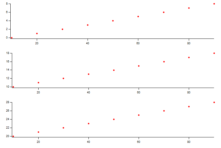
Multiple Y-Formulas¶

Several y-formulas can be plotted with the keyword with. The with must be on an own line between the y-formulas. If the y-data contains different data units the y-axis will show all data units separated by /. The vs allows to set a custom x-formula for the single y-formula left to it. Variables, see next section, can be used to reuse x-formulas for multiple statements without code duplication.

xdata = range(10, 100, 10)

0...10
with
20...30 vs $xdata
and
30...40
with
40...50 vs $xdata

Variables¶

Variables store results of expressions. In formulas variables are included as strings prefixed by $. They are specified in the lines before the formula expression. The format of a variable definition is variableName = expression. The variable name must start with a letter. Further allowed letters are alphanumeric and _. The variable names are treated case-insensitive.

c = cursors(A,B)
s = select(channels(AD), sweeps(), all)

data($c, $s)

The section containing the variable definition can contain empty lines. The first line that is not fulfilling the format for a variable definition is treated as the first line of the formula expression(s) section. Variable definitions can use variables that were defined in a preceding line.

c = cursors(A,B)
s = select(channels(AD), sweeps(), all)
d = data($c, $s)

$d

Previous variable content is discarded when the formula notebook is executed.

Limitations of the current variable definition concept:

The expression for a variable definition is resolved to a single wave reference wave
A single variable can not replace multiple arguments of an operation as operation arguments are processed one-at-a-time.

# This does NOT work
c = cursors(A,B)
s = select(channels(AD), sweeps(), all)
p = $c, $s # p is resolved to a single numerical array

data($p) # the data operation sees a single argument

As a general rule of thumb the result of an operation is a single wave reference wave and thus valid for a variable assignment.

Variables are stored in the Data/SweepBrowsers data folder in the variableStorage wave.

Getting Quick Help¶

In the Sweep Formula notebook it is possible to get a quick help for operation and keywords like vs and and. Mark the operation in question with the mouse and hover over it, a tooltip appears that shows the help for this operation. Alternatively hold shift and right-click to jump to the Help tab that shows the help for the marked operation.

Writing Operations¶

The following sketches some templates to write an operation.

Generally the JSON must not be parsed by the operation itself, but the wrapper functions have to be used.

Steps:

Get and check the number of arguments.
Retrieve and check all mandatory arguments. Use SF_GetArgument for arguments that can consist of multiple data waves and SF_GetArgumentSingle for arguments that are expected to return only a single data wave.
Retrieve all optional arguments from last to first and set for each a default value of not present. (see also operation code for setscale)
Create a output waveRef wave with SF_CreateSFRefWave of the correct size.
Execute the operation calculation, typically for each input data wave independently.
Be aware that a data wave might be a null wave, check sanity of input data wave, tranfer scales from input to calculation result if possible
Handle the Meta data, set a data type and transfer the wave notes on demand.
Return the operation result(s) through SF_GetOutputForExecutor or SF_GetOutputForExecutorSingle if the operation has only a single data wave as result.
Add the data type handling in SF_GetTraceColor and SF_GetMetaDataAnnotationText for proper trace colors and legend annotations in the formula plotter.

Example code for a typical operation taking three arguments, the first argument is some kind of input data.

static Function/WAVE SF_OperationTemplate(variable jsonId, string jsonPath, string graph)

       variable numArgs
       string inDataType

       numArgs = SF_GetNumberOfArguments(jsonID, jsonPath) // Get number of arguments 0 to N
       SF_ASSERT(numArgs <=3, "Operation has 3 arguments at most.") // Check if number of arguments is correct
       SF_ASSERT(numArgs > 1, "Operation needs at least two arguments.")

  WAVE/WAVE arg0 = SF_GetArgument(jsonID, jsonPath, graph, SF_OP_OPSHORTNAME, 0) // Get first argument, this getter allows multiple data waves in the argument
  // For easy operation arguments it is good to have only a single argument with multiple data waves

       WAVE arg1 = SF_GetArgumentSingle(jsonID, jsonPath, graph, SF_OP_OPSHORTNAME, 1, checkExist=1) // Get second argument, only a single data wave is expected that must exist
       SF_ASSERT(DimSize(arg1, ROWS) == 1, "Too many input values for argument two") // Sanity checks for second argument
       SF_ASSERT(IsNumericWave(arg1), "opName argument two must be numeric")

  // Parse optional arguments from last to first
       if(numArgs == 3)
               WAVE arg2 = SF_GetArgumentSingle(jsonID, jsonPath, graph, SF_OP_OPSHORTNAME, 2, checkExist=1)
               SF_ASSERT(DimSize(arg2, ROWS) == 1, "Too many input values for parameter edge")
               SF_ASSERT(IsNumericWave(arg2), "edge parameter must be numeric")
       else
     // Set default value for optional argument if not existing
               Make/FREE edge = {FINDLEVEL_EDGE_BOTH}
       endif

  // Create output wave
       WAVE/WAVE output = SF_CreateSFRefWave(graph, SF_OP_OPSHORTNAME, DimSize(arg0, ROWS))
       output = OperationCalculation(arg0[p], arg1[0], arg2[0])

  // Handle meta data
  // Set data type and transfer sweep information if input data was of the correct type

       SetStringInJSONWaveNote(results, SF_META_DATATYPE, SF_DATATYPE_THISOP)
       inDataType = GetStringFromJSONWaveNote(dataRef, SF_META_DATATYPE)
       if(!CmpStr(inDataType, SF_DATATYPE_SWEEP))
               SF_TransferFormulaDataWaveNote(arg0, output, "Sweeps", SF_META_SWEEPNO)
       endif

  // Return multiple data waves to executor, the function will wrap the wave ref wave to a one element text wave
       return SF_GetOutputForExecutor(results, graph, SF_OP_OPSHORTNAME)
End

static Function/WAVE OperationCalculation(WAVE/Z input, variable arg1, variable arg2)

       if(!WaveExists(input))
               return $""
       endif

  // Sanity checks on input data waves
       SF_ASSERT(IsNumericWave(input), "opname requires numeric data as input")
       SF_ASSERT(WaveDims(input) <= 2, "opname accepts only upto 2d data")
       SF_ASSERT(DimSize(input, ROWS) > 0, "opname requires at least one data point")
       // Do the actual calculation
  MatrixOP/FREE out = sqrt(averageCols(magsqr(input)))^t
  // Transfer the scaling if possible
       SF_FormulaWaveScaleTransfer(input, out, COLS, ROWS)

       return out
End

Example code for an operation taking the top array as input data. The specific difference here is that we use a convention that if there is only a single argument then we parse it as it could possibly an argument with multiple data waves. If it is just regular data then it is converted to a single data wave with one element and thus, stays compatible with the SF_GetArgumentTop parsing, if that would have encountered a single element. This allows to put output from e.g. data directly in such an operation as first argument. The operation works then on each data wave separately.

 static Function/WAVE SF_OperationTemplate(variable jsonId, string jsonPath, string graph)

        variable numArgs

        numArgs = SF_GetNumberOfArguments(jsonId, jsonPath)
        if(numArgs > 1)
                WAVE/WAVE input = SF_GetArgumentTop(jsonId, jsonPath, graph, SF_OP_OPSHORTNAME)
        else
                WAVE/WAVE input = SF_GetArgument(jsonId, jsonPath, graph, SF_OP_OPSHORTNAME, 0)
        endif
        WAVE/WAVE output = SF_CreateSFRefWave(graph, SF_OP_OPSHORTNAME, DimSize(input, ROWS))

        output[] = OperationCalculation(input[p])

        SFH_TransferFormulaDataWaveNoteAndMeta(input, output, SF_OP_OPSHORTNAME, SF_DATATYPE_OP)

        return SF_GetOutputForExecutor(output, graph, SF_OP_OPSHORTNAME, clear=input)
End

static Function/WAVE OperationCalculation(WAVE/Z input)

  // data waves can be null
       if(!WaveExists(input))
              return $""
       endif

       SF_ASSERT(IsNumericWave(input), "opName requires numeric input data.")
       SF_ASSERT(DimSize(input, ROWS) > 0, "opName input must have at least one data point")
  // Do actual calculation
       WAVE out = NewFreeWave(IGOR_TYPE_64BIT_FLOAT, 0)
       Integrate/METH=1/DIM=(ROWS) input/D=out
  // Transfer scales and adapt
       CopyScales input, out
       SetScale/P x, DimOffset(input, ROWS), DimDelta(input, ROWS), "dx", out

       return out
End

The function SFH_TransferFormulaDataWaveNoteAndMeta transfers the meta information and wave notes of the reference and data waves. It also updates the operation stack information. There are two cases where SFH_TransferFormulaDataWaveNoteAndMeta can not be used:

The operation does not take an input reference wave
The operation returns data through SF_GetOutputForExecutorSingle that creates the reference wave.

For operation that do not take an input reference wave that is calculated to an output reference wave the approach is to update the operation stack meta information directly through JWN_SetStringInWaveNote(output, SF_META_OPSTACK, AddListItem(SF_OP_OPSHORT, “”)). If SF_GetOutputForExecutorSingle is called then the optional parameter opStack should be set to the previous operation stack. For operations like sweeps() there is no previous operation, thus the parameter would be opStack=””.

It should be noted that there is a difference for parsing a single first argument through SF_GetArgument or SF_GetArgumentTop. SF_GetArgument starts execution for argument 0 specifically at the /0 JSON path location, whereas SF_GetArgumentTop starts execution at /. Set the case that the first argument is wave(pathToWave) with a 1d-wave containing a single element with value 17. SF_GetArgument executes the wave operation first, whereas SF_GetArgumentTop executes the array [wave(pathToWave)] first. Thus, SF_GetArgument sees with the resolved wave operation [17], whereas SF_GetArgumentTop sees [[17]]. Therefore the first returns a {17} wave and the latter a {{17}} wave.

More complex operation such as data build the output wave reference wave dynamically. See SF_GetSweepsForFormula how the output wave is build depending on selectData and the found sweeps.

Meta Data Handling¶

Operation as well as the formula plotter can evaluate returned meta data from the result wave(s). Generally meta data is set through JSON wave notes. Data wave independent meta data is set in the wave ref wave, whereas data wave dependent data is set as note of the data wave(s) itself. Currently certain key constants for meta data fields are defined.

For the wave ref wave:

SF_META_DATATYPE: string, data type of operation result (some operations are transparent for that)
SF_META_XAXISLABEL: string, suggested label for the x-axis for the plotter, typically combined with x-value meta data in the data wave(s)
SF_META_YAXISLABEL: string, suggested label for the y-axis for the plotter
SF_META_OPSTACK: string, tracks the operation stack

For the data wave(s):

SF_META_SWEEPNO: number, number of the sweep that provided the source data
SF_META_CHANNELTYPE: number, channel type from the sweep that provided the source data
SF_META_CHANNELNUMBER: number, channel number from the sweep that provided the source data
SF_META_XVALUES: wave, suggested x-wave for the plotter to display this data wave

See also SF_OperationLabnotebookImpl, where such meta data is set.

The function SFH_TransferFormulaDataWaveNoteAndMeta transfers meta data from one operation to the next. If the following conditions are met then a suggested X-values are set in the meta data:

The input data type is SF_DATATYPE_SWEEP and all output data waves have no wave units for x set and all output data waves have only one data point -> sweep number is set as X-value and “Sweeps” as x label
For any not above specified input data type: if all output data wave have one data point and all output data waves have no wave units for x set and the input data wave has a sweep number value set in the meta data -> sweep number is set as X-value and “Sweeps” as x label

min(
  butterworth(
    integrate(
      derivative(
        data(TP,select(channels(AD0), 4...11,all))
      )
    )
  ,4,100,4)
)

In the above example the data operation sets sweep number as meta data. The SFH_TransferFormulaDataWaveNoteAndMeta function transfers that meta data also to the results of the outer operations. The data waves returned from the min operation contain only a single data point and the result complies with the second set of conditions mentioned above. Thus, the results are displayed in the plotter with sweep numbers on the x-axis and “Sweeps” as x-label.

Operation Stack¶

The operation stack meta data is updated in the called operation, typically through SFH_TransferFormulaDataWaveNoteAndMeta. It is a semicolon separated list of operations called for a single formula, where the most recent operation is at the front of the list. Operations where data from several sources is joined, like plus discard the previous operation stack. Thus, the operation stack contains only operations that were relevant for the strands of data that reaches ultimately the formula plotter. The operation stack information is used to create the trace legend(s) in the graph(s) as well as for the trace names. Also the trace color is determined through evaluation of the operation stack. For example, only if the operation stack indicates that the most recent data originated from a data() operation without intermediate operations that break this data strand, such as +, then the meta iformation about sweep data is taken to determine the traces color.

Argument Setup Stack¶

The idea of the argument setup stack is to store the arguments of each operation to be able determine differences between formulas in the end. This information can be used to change the trace style for differently setup formulas when plotted in the same graph with the with keyword. Also in the legend it can be shown what was setup differently. Operations can prepare argument setup information through a key/value style text wave with two columns. The wave is created with SFH_GetNewArgSetupWave and is filled then by the operation e.g.:

WAVE/T argSetup = SFH_GetNewArgSetupWave(5)

argSetup[0][%KEY] = "Method"
argSetup[0][%VALUE] = SF_OperationApFrequencyMethodToString(method)
argSetup[1][%KEY] = "Level"
argSetup[1][%VALUE] = num2str(level)
argSetup[2][%KEY] = "ResultType"
argSetup[2][%VALUE] = timeFreq
argSetup[3][%KEY] = "Normalize"
argSetup[3][%VALUE] = normalize
argSetup[4][%KEY] = "XAxisType"
argSetup[4][%VALUE] = xAxisType

This information is stored when SFH_TransferFormulaDataWaveNoteAndMeta is called with the optional argSetup argument. If not setup by the operation, by default the only argSetup entry is the operation short name. Thus, the information content without setting it up is the same as in the operation stack.

The information is evaluated in the Formula Plotter to determine if traces from different formulas specified through the with keyword need to be shown with a different marker or line style. It also adapts the legend to show details about differences in arguments in formulas.

apfrequency(data(ST, select(channels(AD), sweeps(), all)), 3, 100, freq, normoversweepsavg, count)
with
apfrequency(data(ST, select(channels(AD), sweeps(), all)), 3, 100, time, norminsweepsavg, count)