Tutorial: Multi-Population Recurrent Network (with BioNet)

Here we will create a heterogenous yet relatively small network consisting of hundreds of recurrently-connected cells. All cells will belong to one of four “cell-types”. Two of these cell types will be biophysically-detailed cells, i.e. containing a full morphology and somatic and dendritic channels and receptors. The other two will be point-neuron models, which lack a full morphology or channels but still provide inhibitory and excitatory activity.

As input to drive the simulation, we will also create an external network of “virtual cells” that synapse directly onto our internal cells and provide spike trains as stimuli.

Note - scripts and files for running this tutorial can be found in the directory sources/chapter04/.

requirements:

• bmtk

• NEURON 7.4+

For more information on the BioNet Simulator, please see the BioNet Overview.

For more information on BMTK and SONATA format, please see the Overview of BMTK and Network Builder pages.

1. Building the network

Set nodes

This network will loosely resemble a portion of one layer in the mouse primary visual cortex (area V1). (See Arkhipov et al., 2018 for an example of a scientific study using a similar system, although with many more cells). Along the center of the column will be a population of 50 biophysically detailed neurons: 80 excitatory Scnn1a cells and 20 inhibitory PV cells.

import numpy as np

from bmtk.builder.networks import NetworkBuilder
from bmtk.builder.auxi.node_params import positions_columinar, xiter_random

net = NetworkBuilder("V1")
net.add_nodes(
    N=80, pop_name='Scnn1a',
    positions=positions_columinar(N=80, center=[0, 50.0, 0], max_radius=30.0, height=100.0),
    rotation_angle_yaxis=xiter_random(N=80, min_x=0.0, max_x=2*np.pi),
    rotation_angle_zaxis=xiter_random(N=80, min_x=0.0, max_x=2*np.pi),
    tuning_angle=np.linspace(start=0.0, stop=360.0, num=80, endpoint=False),
    location='VisL4',
    ei='e',
    model_type='biophysical',
    model_template='ctdb:Biophys1.hoc',
    model_processing='aibs_perisomatic',
    dynamics_params='472363762_fit.json',
    morphology='Scnn1a_473845048_m.swc'
)

net.add_nodes(
    N=20, pop_name='PV',
    positions=positions_columinar(N=20, center=[0, 50.0, 0], max_radius=30.0, height=100.0),
    rotation_angle_yaxis=xiter_random(N=20, min_x=0.0, max_x=2*np.pi),
    rotation_angle_zaxis=xiter_random(N=20, min_x=0.0, max_x=2*np.pi),
    location='VisL4',
    ei='i',
    model_type='biophysical',
    model_template='ctdb:Biophys1.hoc',
    model_processing='aibs_perisomatic',
    dynamics_params='472912177_fit.json',
    morphology='Pvalb_470522102_m.swc'
)

To set the position and rotation of each cell, we use the builtiin functions positions_columinar and xiter_random, which return a list of position and rotation values, respectively. A user could set the values themselves using a list of size N, where N represents the number of cells. The parameters like location, ei, model_type, etc. are cell-type parameters, and will be used for all N cells of that type. See tutorial 2 and tutorial 3 for more details.

The excitatory cells are also given a tuning_angle parameter. The “tuning angle” is an intrinsic property found in some cells in the visual cortex. In this model, we will use this property to determine the strength of connections between subsets of cells by using custom functions. In general most models will not have or use a tuning angle, but they may require some other parameter. Users can assign whatever custom parameters they want to cells and cell-types and use them as properties for creating connections and running simulations.

Next we continue to create our point (integrate-and-fire) neurons. Notice they don’t have properties like rotation_angle_yaxis or morphology, as these don’t apply to point neurons.

net.add_nodes(
    N=200, pop_name='LIF_exc',
    positions=positions_columinar(N=200, center=[0, 50.0, 0], min_radius=30.0, max_radius=60.0, height=100.0),
    tuning_angle=np.linspace(start=0.0, stop=360.0, num=200, endpoint=False),
    location='VisL4',
    ei='e',
    model_type='point_process',
    model_template='nrn:IntFire1',
    dynamics_params='IntFire1_exc_1.json'
)

net.add_nodes(
    N=100, pop_name='LIF_inh',
    positions=positions_columinar(N=100, center=[0, 50.0, 0], min_radius=30.0, max_radius=60.0, height=100.0),
    location='VisL4',
    ei='i',
    model_type='point_process',
    model_template='nrn:IntFire1',
    dynamics_params='IntFire1_inh_1.json'
)

Set edges

Now we want to create connections between the cells. Depending on the model type, and whether or not the presynaptic “source” cell is excitory or inhibitory, we will use different synaptic models and parameters. Using the source and target filter parameters, we can create different connection types.

To determine the excitatory-to-excitatory connection matrix we want to use the distance and tuning_angle properties. To do this we create a customized function dist_tuning_connector:

import random
import math

def dist_tuning_connector(source, target, d_weight_min, d_weight_max, d_max, t_weight_min, t_weight_max, nsyn_min,
                          nsyn_max):
    if source['node_id'] == target['node_id']:
        # Avoid self-connections.n_nodes
        return None

    r = np.linalg.norm(np.array(source['positions']) - np.array(target['positions']))
    if r > d_max:
        dw = 0.0
    else:
        t = r / d_max
        dw = d_weight_max * (1.0 - t) + d_weight_min * t

    if dw <= 0:
        # drop the connection if the weight is too low
        return None

    # next create weights by orientation tuning [ aligned, misaligned ] --> [ 1, 0 ], Check that the orientation
    # tuning property exists for both cells; otherwise, ignore the orientation tuning.
    if 'tuning_angle' in source and 'tuning_angle' in target:

        # 0-180 is the same as 180-360, so just modulo by 180
        delta_tuning = math.fmod(abs(source['tuning_angle'] - target['tuning_angle']), 180.0)

        # 90-180 needs to be flipped, then normalize to 0-1
        delta_tuning = delta_tuning if delta_tuning < 90.0 else 180.0 - delta_tuning

        t = delta_tuning / 90.0
        tw = t_weight_max * (1.0 - t) + t_weight_min * t
    else:
        tw = dw

    # drop the connection if the weight is too low
    if tw <= 0:
        return None

    # filter out nodes by treating the weight as a probability of connection
    if random.random() > tw:
        return None

    # Add the number of synapses for every connection.
    # It is probably very useful to take this out into a separate function.
    return random.randint(nsyn_min, nsyn_max)

The first two parameters of this function are “source” and “target” and are required for all custom connector functions. These are node objects which give a representation of a single source and target cell, with properties that can be accessed like a python dictionary. When The Network Builder creates the connection matrix, it will call this function for all possible source-target pairs. The user doesn’t call this function directly.

The remaining parameters are optional. Using these parameters, plus the distance and angles between source and target cells, this function determines the number of connections between each given source and target cell. If there are none you can return either None or 0.

To create these connections we call the add_edges method of the builder. We use the source and target parameter to filter out only excitatory-to-excitatory connections. We must also take into consideration the model type (biophysical or integrate-and-fire) of the target when setting parameters. We pass in the function through the connection_rule parameter, and the function parameters (except source and target) through connection_params. (If our dist_tuning_connector function didn’t have any parameters other than source and target, we could just not set connection_params).

The parameter weight_function will be described in detail in Step 3.

See tutorial 2 and tutorial 3 for more details.

net.add_edges(
    source={'ei': 'e'}, target={'pop_name': 'Scnn1a'},
    connection_rule=dist_tuning_connector,
    connection_params={'d_weight_min': 0.0, 'd_weight_max': 0.34, 'd_max': 300.0, 't_weight_min': 0.5,
                       't_weight_max': 1.0, 'nsyn_min': 3, 'nsyn_max': 7},
    syn_weight=5e-05,
    weight_function='gaussianLL',
    weight_sigma=50.0,
    distance_range=[30.0, 150.0],
    target_sections=['basal', 'apical'],
    delay=2.0,
    dynamics_params='AMPA_ExcToExc.json',
    model_template='exp2syn'
)

net.add_edges(
    source={'ei': 'e'}, target={'pop_name': 'LIF_exc'},
    connection_rule=dist_tuning_connector,
    connection_params={'d_weight_min': 0.0, 'd_weight_max': 0.34, 'd_max': 300.0, 't_weight_min': 0.5,
                       't_weight_max': 1.0, 'nsyn_min': 3, 'nsyn_max': 7},
    syn_weight=0.0019,
    weight_function='gaussianLL',
    weight_sigma=50.0,
    delay=2.0,
    dynamics_params='instantaneousExc.json',
    model_template='exp2syn'
)

<bmtk.builder.connection_map.ConnectionMap at 0x7f56031b5130>

We create the other types of connections in a similar manner. But since either the source, target, or both cells will not have the tuning_angle parameter, we don’t want to use dist_tuning_connector. Instead we can use the built-in distance_connector function which just creates connections determined by distance.

from bmtk.builder.auxi.edge_connectors import distance_connector

### Generating I-to-I connections
net.add_edges(
    source={'ei': 'i'}, target={'ei': 'i', 'model_type': 'biophysical'},
    connection_rule=distance_connector,
    connection_params={'d_weight_min': 0.0, 'd_weight_max': 1.0, 'd_max': 160.0, 'nsyn_min': 3, 'nsyn_max': 7},
    syn_weight=0.0002,
    weight_function='wmax',
    distance_range=[0.0, 1e+20],
    target_sections=['somatic', 'basal'],
    delay=2.0,
    dynamics_params='GABA_InhToInh.json',
    model_template='exp2syn'
)

net.add_edges(
    source={'ei': 'i'}, target={'ei': 'i', 'model_type': 'point_process'},
    connection_rule=distance_connector,
    connection_params={'d_weight_min': 0.0, 'd_weight_max': 1.0, 'd_max': 160.0, 'nsyn_min': 3, 'nsyn_max': 7},
    syn_weight=0.001,
    weight_function='wmax',
    delay=2.0,
    dynamics_params='instantaneousInh.json',
    model_template='exp2syn'
)

### Generating I-to-E connections
net.add_edges(
    source={'ei': 'i'}, target={'ei': 'e', 'model_type': 'biophysical'},
    connection_rule=distance_connector,
    connection_params={'d_weight_min': 0.0, 'd_weight_max': 1.0, 'd_max': 160.0, 'nsyn_min': 3, 'nsyn_max': 7},
    syn_weight=0.0001,
    weight_function='wmax',
    distance_range=[0.0, 50.0],
    target_sections=['somatic', 'basal', 'apical'],
    delay=2.0,
    dynamics_params='GABA_InhToExc.json',
    model_template='exp2syn'
)

net.add_edges(
    source={'ei': 'i'}, target={'ei': 'e', 'model_type': 'point_process'},
    connection_rule=distance_connector,
    connection_params={'d_weight_min': 0.0, 'd_weight_max': 1.0, 'd_max': 160.0, 'nsyn_min': 3, 'nsyn_max': 7},
    syn_weight=0.009,
    weight_function='wmax',
    delay=2.0,
    dynamics_params='instantaneousInh.json',
    model_template='exp2syn'
)

### Generating E-to-I connections
net.add_edges(
    source={'ei': 'e'}, target={'pop_name': 'PV'},
    connection_rule=distance_connector,
    connection_params={'d_weight_min': 0.0, 'd_weight_max': 0.26, 'd_max': 300.0, 'nsyn_min': 3, 'nsyn_max': 7},
    syn_weight=0.004,
    weight_function='wmax',
    distance_range=[0.0, 1e+20],
    target_sections=['somatic', 'basal'],
    delay=2.0,
    dynamics_params='AMPA_ExcToInh.json',
    model_template='exp2syn'
)

net.add_edges(
    source={'ei': 'e'}, target={'pop_name': 'LIF_inh'},
    connection_rule=distance_connector,
    connection_params={'d_weight_min': 0.0, 'd_weight_max': 0.26, 'd_max': 300.0, 'nsyn_min': 3, 'nsyn_max': 7},
    syn_weight=0.006,
    weight_function='wmax',
    delay=2.0,
    dynamics_params='instantaneousExc.json',
    model_template='exp2syn'
)

<bmtk.builder.connection_map.ConnectionMap at 0x7f5602eec400>

Finally we build the network (this may take a bit of time since there are many possible connection combinations), and save the nodes and edges.

net.build()
net.save_nodes(output_dir='sim_ch04/network')
net.save_edges(output_dir='sim_ch04/network')

Build external network

Next we want to create an external network consisting of virtual cells that form a feedforward network onto our V1, which will provide input during the simulation. We will call this LGN, since the LGN is the primary input to layer 4 cells of the V1 (if we wanted to we could also create multiple external networks and run simulations on any number of them).

First we build our LGN nodes. Then we must import the V1 network nodes and create connections from LGN to V1.

from bmtk.builder.networks import NetworkBuilder

lgn = NetworkBuilder('LGN')
lgn.add_nodes(
    N=500,
    pop_name='tON',
    potential='exc',
    model_type='virtual'
)

As before, we will use a customized function to determine the number of connections between each source and target pair, however this time our connection rule is a bit different.

In the previous example our connection rule function’s first two arguments were the presynaptic and postsynaptic cells, which allowed us to choose the number of synaptic connections between pairs based on individual properties:

def connection_fnc(source, target, ...):
    source['param'] # presynaptic cell params
    target['param'] # postsynaptic cell params
    ...
    return nsyns # number of connections between pair

But for our LGN –> V1 connection, we do things a bit differently. We want to make sure that for every source cell, there are a limited number of presynaptic targets. This is a not really possible with a function that iterates on a one-to-one basis. So instead we have a connector function for which the first parameter is a list of all N source cell while the second parameter is a single target cell. We return an array of integers, size N, with each element representing the number of synapses between the sources and the target.

To tell the builder to use this schema, we must set iterator='all_to_one' in the add_edges method. (By default this is set to ‘one_to_one’. You can also use ‘one_to_all’ iterator which will pass in a single source and all possible targets).

def select_source_cells(sources, target, nsources_min=10, nsources_max=30, nsyns_min=3, nsyns_max=12):
    total_sources = len(sources)
    nsources = np.random.randint(nsources_min, nsources_max)
    selected_sources = np.random.choice(total_sources, nsources, replace=False)
    syns = np.zeros(total_sources)
    syns[selected_sources] = np.random.randint(nsyns_min, nsyns_max, size=nsources)
    return syns

lgn.add_edges(
    source=lgn.nodes(), target=net.nodes(pop_name='Scnn1a'),
    iterator='all_to_one',
    connection_rule=select_source_cells,
    connection_params={'nsources_min': 10, 'nsources_max': 25},
    syn_weight=1e-03,
    weight_function='wmax',
    distance_range=[0.0, 150.0],
    target_sections=['basal', 'apical'],
    delay=2.0,
    dynamics_params='AMPA_ExcToExc.json',
    model_template='exp2syn'
)

lgn.add_edges(
    source=lgn.nodes(), target=net.nodes(pop_name='PV1'),
    connection_rule=select_source_cells,
    connection_params={'nsources_min': 15, 'nsources_max': 30},
    iterator='all_to_one',
    syn_weight=0.015,
    weight_function='wmax',
    distance_range=[0.0, 1.0e+20],
    target_sections=['somatic', 'basal'],
    delay=2.0,
    dynamics_params='AMPA_ExcToInh.json',
    model_template='exp2syn'
)

lgn.add_edges(
    source=lgn.nodes(),  target=net.nodes(pop_name='LIF_exc'),
    connection_rule=select_source_cells,
    connection_params={'nsources_min': 10, 'nsources_max': 25},
    iterator='all_to_one',
    syn_weight= 0.07,
    weight_function='wmax',
    delay=2.0,
    dynamics_params='instantaneousExc.json',
    model_template='exp2syn'
)

lgn.add_edges(
    source=lgn.nodes(),  target=net.nodes(pop_name='LIF_inh'),
    connection_rule=select_source_cells,
    connection_params={'nsources_min': 15, 'nsources_max': 30},
    iterator='all_to_one',
    syn_weight=0.05,
    weight_function='wmax',
    delay=2.0,
    dynamics_params='instantaneousExc.json',
    model_template='exp2syn'
)

lgn.build()
lgn.save_nodes(output_dir='sim_ch04/network')
lgn.save_edges(output_dir='sim_ch04/network')

2. Setting up BioNet

File structure

Before running a simulation, we will need to create the runtime environment, including parameter files, run-script and configuration files. You can copy the files from an existing simulation and execute with the following command:

$ python -m bmtk.utils.sim_setup  \
   --report-vars v                \
   --report-nodes 10,80           \
   --network sim_ch04/network     \
   --dt 0.1                       \
   --tstop 3000.0                 \
   --include-examples             \
   --compile-mechanisms           \
   bionet sim_ch04

$ python -m bmtk.utils.sim_setup –report-vars v –report-nodes 0,80,100,300 –network sim_ch04/network –dt 0.1 –tstop 3000.0 –include-examples –compile-mechanisms bionet sim_ch04

or run it directly in python:

from bmtk.utils.sim_setup import build_env_bionet

build_env_bionet(
    base_dir='sim_ch04',
    config_file='config.json',
    network_dir='sim_ch04/network',
    tstop=3000.0, dt=0.1,
    report_vars=['v'],     # Record membrane potential (default soma)
    include_examples=True,    # Copies components files
    compile_mechanisms=True   # Will try to compile NEURON mechanisms
)

This will fill out the sim_ch04 with all the files we need to get started to run the simulation. Of interest includes

• circuit_config.json - A configuration file that contains the location of the network files we created above. Plus location of neuron and synaptic models, templates, morphologies and mechanisms required to build our circuit and instantiate individual cell models.

• simulation_config.json - contains information about the simulation. Including initial conditions and run-time configuration (run and conditions). In the inputs section we define what external sources we will use to drive the network (in this case a current clamp). And in the reports section we define the variables (soma membrane potential and calcium) that will be recorded during the simulation

• run_bionent.py - A script for running our simulation. Usually this file doesn’t need to be modified.

• components/biophysical_neuron_models/ - The parameter file for the cells we’re modeling. Originally downloaded from the Allen Cell Types Database. These files were automatically copied over when we used the include-examples directive. If using a differrent or extended set of cell models place them here

• components/biophysical_neuron_models/ - The morphology file for our cells. Originally downloaded from the Allen Cell Types Database and copied over using the include_examples.

• components/point_neuron_models/ - The parameter file for our LIF_exc and LIF_inh cells.

• components/synaptic_models/ - Parameter files used to create different types of synapses.

LGN Input

We need to provide our LGN external network cells with spike-trains so they can activate our recurrent network. Previously we showed how to do this by generating CSV files. We can also use NWB files, which are a common format for saving electrophysiological data in neuroscience.

We can use any NWB file generated experimentally or computationally, but for this example we will use a pre-existing file. First download the file:

$ wget https://github.com/AllenInstitute/bmtk/blob/develop/examples/spikes_inputs/lgn_spikes.h5?raw=true -O lgn_spikes.h5

or copy from here.

Then we must edit the simulation_config.json file to tell the simulator where to find the spike file and which network to associate it with:

{
  "inputs": {
    "LGN_spikes": {
      "input_type": "spikes",
      "module": "sonata",
      "input_file": "$BASE_DIR/lgn_spikes.h5",
      "node_set": "LGN"
    }
  }
}

3. Running the simulation

We are close to running our simulation, however unlike previous chapters we need a little more programming before we can begin.

For most of the connections we added the parameter weight_function='wmax'. This is a built-in function that tells the simulator to use the ‘weight_max’ value assigned to that edge-type when creating a connection between two cells.

However, when creating excitatory-to-excitatory connections we want to use the weight_function='gaussianLL'. This is because we want to use the ‘tuning_angle’ parameter, when available, to determine the synaptic strength between two connections. First we create the function which takes in target, source and connection properties (which are just the edge-type and properties set in the add_edges method). Then we must register the function with the BioNet simulator:

import math
from bmtk.simulator.bionet.pyfunction_cache import add_weight_function

def gaussianLL(edge_props, source, target):
    src_tuning = source['tuning_angle']
    tar_tuning = target['tuning_angle']
    w0 = edge_props["syn_weight"]
    sigma = edge_props["weight_sigma"]

    delta_tuning = abs(abs(abs(180.0 - abs(float(tar_tuning) - float(src_tuning)) % 360.0) - 90.0) - 90.0)
    return w0 * math.exp(-(delta_tuning / sigma) ** 2)

add_weight_function(gaussianLL)

The weights will be adjusted before each simulation, and the function can be changed between different runs. Simply opening the edge_types.csv file with a text editor and altering the weight_function column allows users to take an existing network and readjust weights as needed in each new simulation runtime.

Finally we are ready to run the simulation. Note that because this is a 400 cell simulation, this may be computationally intensive for some older computers and may take anywhere between a few minutes to half-an-hour to complete.

from bmtk.simulator import bionet


conf = bionet.Config.from_json('sim_ch04/config.json')
conf.build_env()
net = bionet.BioNetwork.from_config(conf)
sim = bionet.BioSimulator.from_config(conf, network=net)
sim.run()

2022-11-01 16:23:09,716 [INFO] Created log file

INFO:NEURONIOUtils:Created log file

numprocs=1
2022-11-01 16:23:09,800 [INFO] Building cells.

INFO:NEURONIOUtils:Building cells.

2022-11-01 16:23:17,484 [INFO] Building recurrent connections

INFO:NEURONIOUtils:Building recurrent connections

2022-11-01 16:23:36,637 [INFO] Building virtual cell stimulations for LGN_spikes

INFO:NEURONIOUtils:Building virtual cell stimulations for LGN_spikes

2022-11-01 16:23:38,276 [INFO] Running simulation for 3000.000 ms with the time step 0.100 ms

INFO:NEURONIOUtils:Running simulation for 3000.000 ms with the time step 0.100 ms

2022-11-01 16:23:38,277 [INFO] Starting timestep: 0 at t_sim: 0.000 ms

INFO:NEURONIOUtils:Starting timestep: 0 at t_sim: 0.000 ms

2022-11-01 16:23:38,278 [INFO] Block save every 5000 steps

INFO:NEURONIOUtils:Block save every 5000 steps

2022-11-01 16:24:19,186 [INFO]     step:5000 t_sim:500.00 ms

INFO:NEURONIOUtils:    step:5000 t_sim:500.00 ms

2022-11-01 16:25:02,737 [INFO]     step:10000 t_sim:1000.00 ms

INFO:NEURONIOUtils:    step:10000 t_sim:1000.00 ms

2022-11-01 16:25:44,100 [INFO]     step:15000 t_sim:1500.00 ms

INFO:NEURONIOUtils:    step:15000 t_sim:1500.00 ms

2022-11-01 16:26:30,819 [INFO]     step:20000 t_sim:2000.00 ms

INFO:NEURONIOUtils:    step:20000 t_sim:2000.00 ms

2022-11-01 16:27:13,897 [INFO]     step:25000 t_sim:2500.00 ms

INFO:NEURONIOUtils:    step:25000 t_sim:2500.00 ms

2022-11-01 16:27:56,117 [INFO]     step:30000 t_sim:3000.00 ms

INFO:NEURONIOUtils:    step:30000 t_sim:3000.00 ms

2022-11-01 16:27:56,176 [INFO] Simulation completed in 4.0 minutes, 17.9 seconds

INFO:NEURONIOUtils:Simulation completed in 4.0 minutes, 17.9 seconds

4. Analyzing results

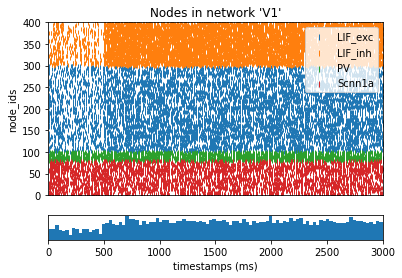
Results of the simulation are saved into the output directory, as specified in the config file. Using the analyzer functions, we can do things like plot the raster plot:

from bmtk.analyzer.spike_trains import plot_raster, plot_rates_boxplot

_ = plot_raster(config_file='sim_ch04/config.json', group_by='pop_name')

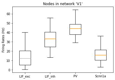
and the rates of each node:

_ = plot_rates_boxplot(config_file='sim_ch04/config.json', group_by='pop_name')

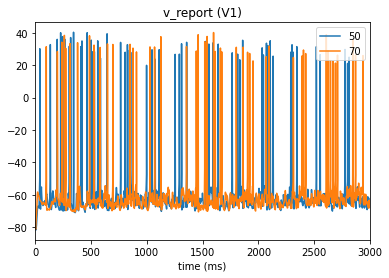
In our config file we used the cell_vars and node_id_selections parameters to save the calcium influx and membrane potential of selected cells. We can also use the analyzer to display these traces:

from bmtk.analyzer.compartment import plot_traces

_ = plot_traces(config_file='sim_ch04/config.json', report_name='v_report', node_ids=[50,70])