Tutorial: Multi-Cell, Single Population Network (with BioNet)#
In this tutorial, we will create a more complex network that contains multiple biophysical cells of the same cell-type (we will cover heterogenous networks in the next tutorial). The network will contain recurrent connections, as well as external input that provides input to the network.
Note - scripts and files for running this tutorial can be found in the directory sources/chapter03/
requirements:
bmtk
NEURON 7.4+
For more information on the BioNet Simulator, please see the BioNet Overview.
For more information on BMTK and SONATA format, please see the Overview of BMTK and Network Builder pages.
1. Building the Network#
First we will build our internal network, which consists of 100 different cells. All the cells are of the same type but they all have a different location and y-axis rotation.
Set nodes#
[1]:
import numpy as np
from bmtk.builder.networks import NetworkBuilder
from bmtk.builder.auxi.node_params import positions_columinar, xiter_random

cortex = NetworkBuilder('mcortex')
cortex.add_nodes(
    N=100,
    pop_name='Scnn1a',
    positions=positions_columnar(N=100, center=[0, 50.0, 0], max_radius=30.0, height=100.0),
    rotation_angle_yaxis=xiter_random(N=100, min_x=0.0, max_x=2*np.pi),
    rotation_angle_zaxis=3.646878266,
    potental='exc',
    model_type='biophysical',
    model_template='ctdb:Biophys1.hoc',
    model_processing='aibs_perisomatic',
    dynamics_params='472363762_fit.json',
    morphology='Scnn1a_473845048_m.swc'
)
New parameters:
N - Indicates the number of cells in our population.
positions - Sets the spatial location of each cell in the network. Here we define it by the
positions_columnarbuilt-in method, which will randomly place our cells in a column (users can define their own positions as shown here).rotation_angle_yaxis - Sets the y angle for each cell. Here it is defined by a built-in function
xiter_randomthat randomly assigns each cell a given y angle.rotation_angle_zaxis - Sets the z angle for each cell. Here we assign a single value to each cell.
See tutorial 1 for a description of the other parameters.
Note - Here we define the y-angle (that is, the angle or rotation around the y-axis) by a function which returns a lists of values, but the z-angle is defined by a single value. This means that all cells will share the z-angle. we could alteratively give all cells the same y-rotation angle:
rotation_angle_yaxis=rotation_value
or give all cells a unique z-rotation angle:
rotation_angle_zaxis=xiter_random(N=100, min_x=0.0, max_x=2*np.pi)
and in general, it is at the discretion of the modeler to choose what parameters are unique to each cell, and what parameters are global to the cell-type.
Set edges#
Next we want to add recurrent edges. To create the connections we will use the built-in distance_connector function, which will assign the number of connections between two cells randomly (in the range nsyn_min and nsysn_max) but weighted by distance. The other parameters, including the synaptic model (AMPA_ExcToExc) will be shared by all connections.
To use this, or to use customized connection functions, we must pass in the name of our connection function using the “connection_rule” parameter, and the function parameters through “connection_params” as a dictionary, which will looks something like:
connection_rule=<name_of_function>
connection_params={'param_arg1': val1, 'param_arg2': val2, ...}
The connection_rule method isn’t explicitly called by the script. Rather when the build() method is called, the connection_rule will iterate through every source/target node pair, and use the rule to build a connection matrix.
See tutorial 2 for a description of the other parameters.
After building the connections based on our connection function, we will save the nodes and edges files into the network/directory.
[2]:
from bmtk.builder.auxi.edge_connectors import distance_connector

cortex.add_edges(
    source={'pop_name': 'Scnn1a'}, target={'pop_name': 'Scnn1a'},
    connection_rule=distance_connector,
    connection_params={'d_weight_min': 0.0, 'd_weight_max': 0.34, 'd_max': 50.0, 'nsyn_min': 0, 'nsyn_max': 10},
    syn_weight=2.0e-04,
    distance_range=[30.0, 150.0],
    target_sections=['basal', 'apical', 'soma'],
    delay=2.0,
    dynamics_params='AMPA_ExcToExc.json',
    model_template='exp2syn'
)
[2]:
<bmtk.builder.connection_map.ConnectionMap at 0x7f89003e26d0>
Build the main network#
[3]:
cortex.build()
cortex.save_nodes(output_dir='sim_ch03/network')
cortex.save_edges(output_dir='sim_ch03/network')
Create the input network#
After building our internal network, we will build the external thalamic network which will provide input (See tutorial 2 for more details). Our thalamic network will consist of 100 “filter” cells, which aren’t actual cells but rather just place holders for spike-trains.
[4]:
thalamus = NetworkBuilder('mthalamus')
thalamus.add_nodes(
    N=100,
    pop_name='tON',
    potential='exc',
    model_type='virtual'
)
The input network doesn’t have recurrent connections, rather all the cells are connected in a feedforward fashion onto the internal network. To connect the networks we create edges with the thalamus nodes as the sources and the cortex nodes as the targets. This time we use the built-in connect_random connection rule, which will randomly assign each thalamus –> cortex connection between 0 and 12 synapses.
Note - If building the input network in a separate script you would need to reload the saved mcortex network cell files using the import function.
[5]:
from bmtk.builder.auxi.edge_connectors import connect_random

thalamus.add_edges(
    source=thalamus.nodes(), target=cortex.nodes(),
    connection_rule=connect_random,
    connection_params={'nsyn_min': 0, 'nsyn_max': 12},
    syn_weight=5.0e-05,
    distance_range=[0.0, 150.0],
    target_sections=['basal', 'apical'],
    delay=2.0,
    dynamics_params='AMPA_ExcToExc.json',
    model_template='exp2syn'
)

thalamus.build()
thalamus.save_nodes(output_dir='sim_ch03/network')
thalamus.save_edges(output_dir='sim_ch03/network')
Spike Trains#
Next we need to create the individual spike trains for our thalamic filter cells. We will use a Poisson distribution of spikes for our 300 cells, each firing at ~ 15 Hz over a 3 second window. Then we can save our spike trains as a SONATA file under the sim_ch03/inputs directory.
[6]:
from bmtk.utils.reports.spike_trains import PoissonSpikeGenerator

psg = PoissonSpikeGenerator(population='mthalamus')
psg.add(node_ids=range(100),  # Have 10 nodes to match mthalamus
        firing_rate=15.0,    # 15 Hz, we can also pass in a nonhomogeneous function/array
        times=(0.0, 3.0))    # Firing starts at 0 s up to 3 s
psg.to_sonata('sim_ch03/inputs/mthalamus_spikes.h5')

# Let's do a quick check that we have reasonable results. Should see somewhere on the order of 15*3*100 = 4500
# spikes
psg.to_dataframe().head()
[6]:
| node_ids | timestamps | population | |
|---|---|---|---|
| 0 | 0 | 87.943425 | mthalamus |
| 1 | 0 | 110.660282 | mthalamus |
| 2 | 0 | 140.897319 | mthalamus |
| 3 | 0 | 170.834006 | mthalamus |
| 4 | 0 | 174.629060 | mthalamus |
2. Setting up BioNet#
File structure#
Before running a simulation, we will need to create the runtime environment, including parameter files, run-script and configuration files. If you’ve already completed tutorial 2 you can just copy the files to sim_ch03 (just make sure not to overwrite the network and inputs directory).
Or create them from scratch by either running the command:
$ python -m bmtk.utils.sim_setup  \
   --report-vars v,cai            \
   --network sim_ch03/network     \
   --spikes-inputs mthalamus:sim_ch03/inputs/mthalamus_spikes.h5 \
   --dt 0.1             \
   --tstop 3000.0       \
   --include-examples   \
   --compile-mechanisms \
   bionet sim_ch03
Or call the function directly in python:
[ ]:
from bmtk.utils.sim_setup import build_env_bionet

build_env_bionet(
    base_dir='sim_ch03',
    config_file='config.json',
    network_dir='sim_ch03/network',
    tstop=3000.0, dt=0.1,
    report_vars=['v', 'cai'],     # Record membrane potential and calcium (default soma)
    spikes_inputs=[('mthalamus',   # Name of population which spikes will be generated for
                    'sim_ch03/inputs/mthalamus_spikes.h5')],
    include_examples=True,    # Copies components files
    compile_mechanisms=True   # Will try to compile NEURON mechanisms
)
It’s a good idea to check the configuration files sim_ch03/circuit_config.json and sim_ch03/simulation_config.json, especially to make sure that bmtk will know to use our generated spikes file (if you don’t see the below section in the simulation_config.json file, go ahead and add it).
{
  "inputs": {
    "tc_spikes": {
      "input_type": "spikes",
      "module": "csv",
      "input_file": "${BASE_DIR}/mthalamus_spikes.csv",
      "node_set": "mthalamus"
    }
  }
}
3. Running the simulation#
Once our config file is setup we can run a simulation either through the command line:
$ cd sim_ch03
$ python run_bionet.py config.json
or through the script:
[8]:
from bmtk.simulator import bionet


conf = bionet.Config.from_json('sim_ch03/config.json')
conf.build_env()
net = bionet.BioNetwork.from_config(conf)
sim = bionet.BioSimulator.from_config(conf, network=net)
sim.run()
2022-08-09 21:44:46,934 [INFO] Created log file
INFO:NEURONIOUtils:Created log file
numprocs=1
2022-08-09 21:44:47,012 [INFO] Building cells.
INFO:NEURONIOUtils:Building cells.
2022-08-09 21:44:54,838 [INFO] Building recurrent connections
INFO:NEURONIOUtils:Building recurrent connections
2022-08-09 21:44:55,189 [INFO] Building virtual cell stimulations for mthalamus_spikes
INFO:NEURONIOUtils:Building virtual cell stimulations for mthalamus_spikes
2022-08-09 21:44:58,773 [INFO] Running simulation for 3000.000 ms with the time step 0.100 ms
INFO:NEURONIOUtils:Running simulation for 3000.000 ms with the time step 0.100 ms
2022-08-09 21:44:58,774 [INFO] Starting timestep: 0 at t_sim: 0.000 ms
INFO:NEURONIOUtils:Starting timestep: 0 at t_sim: 0.000 ms
2022-08-09 21:44:58,775 [INFO] Block save every 5000 steps
INFO:NEURONIOUtils:Block save every 5000 steps
2022-08-09 21:45:26,516 [INFO] step:5000 t_sim:500.00 ms
INFO:NEURONIOUtils: step:5000 t_sim:500.00 ms
2022-08-09 21:45:54,497 [INFO] step:10000 t_sim:1000.00 ms
INFO:NEURONIOUtils: step:10000 t_sim:1000.00 ms
2022-08-09 21:46:26,947 [INFO] step:15000 t_sim:1500.00 ms
INFO:NEURONIOUtils: step:15000 t_sim:1500.00 ms
2022-08-09 21:46:56,036 [INFO] step:20000 t_sim:2000.00 ms
INFO:NEURONIOUtils: step:20000 t_sim:2000.00 ms
2022-08-09 21:47:24,824 [INFO] step:25000 t_sim:2500.00 ms
INFO:NEURONIOUtils: step:25000 t_sim:2500.00 ms
2022-08-09 21:47:55,361 [INFO] step:30000 t_sim:3000.00 ms
INFO:NEURONIOUtils: step:30000 t_sim:3000.00 ms
2022-08-09 21:47:55,393 [INFO] Simulation completed in 2.0 minutes, 56.62 seconds
INFO:NEURONIOUtils:Simulation completed in 2.0 minutes, 56.62 seconds
4. Analyzing the run#
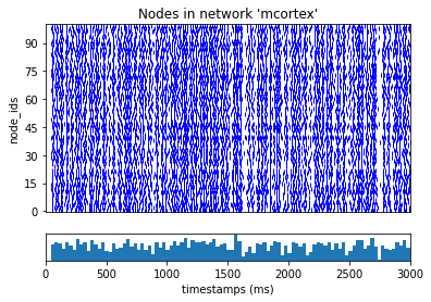
If successful, we should have our results in the output directory. We can use the analyzer to plot a raster of the spikes over time:
[9]:
from bmtk.analyzer.spike_trains import plot_raster


_ = plot_raster(config_file='sim_ch03/config.json')
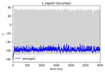
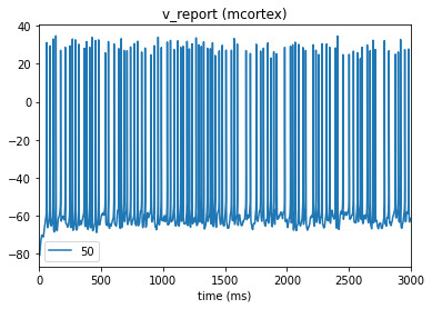
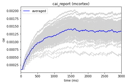
In our config file we used the cell_vars and node_id_selections parameters to save the calcium influx and membrane potential of selected cells. We can also use the analyzer to display these traces:
[10]:
from bmtk.analyzer.compartment import plot_traces

_ = plot_traces(config_file='sim_ch03/config.json', report_name='v_report')
_ = plot_traces(config_file='sim_ch03/config.json', report_name='v_report', node_ids=[50])
_ = plot_traces(config_file='sim_ch03/config.json', report_name='cai_report')
5. Additional Information#
Customized node parameters#
When building our cortex nodes, we used some built-in functions to set certain parameters like positions and y-axis rotations:
cortex.add_nodes(N=100,
                 pop_name='Scnn1a',
                 positions=positions_columinar(N=100, center=[0, 50.0, 0], max_radius=30.0, height=100.0),
                 rotation_angle_yaxis=xiter_random(N=100, min_x=0.0, max_x=2*np.pi),
                 ...
These functions will assign every cell a unique value in the positions and rotation_angle_yaxis parameters, unlike the pop_name parameter which will be the same for all 100 cells. We can verify by the following code:
[11]:
cortex_nodes = list(cortex.nodes())
n0 = cortex_nodes[0]
n1 = cortex_nodes[1]
print('cell 0: pop_name: {}, positions: {}, angle_yaxis: {}'.format(n0['pop_name'], n0['positions'], n0['rotation_angle_yaxis']))
print('cell 1: pop_name: {}, positions: {}, angle_yaxis: {}'.format(n1['pop_name'], n1['positions'], n1['rotation_angle_yaxis']))
cell 0: pop_name: Scnn1a, positions: [-12.67936906  16.99325185  -8.20277884], angle_yaxis: 5.127788634883025
cell 1: pop_name: Scnn1a, positions: [ -1.22804411  91.62129377 -11.58852979], angle_yaxis: 1.0965697825257734
The Network Builder contains a growing number of built-in functions. However for advanced networks a modeler will probably want to assign parameters using their own functions. To do so, a modeler only needs to pass in, or alternatively create a function that returns, a list of size N. When saving the network, each individual position will be saved in the nodes.h5 file assigned to each cell by a unique ID number.
def cortex_positions(N):
    # codex to create a list/numpy array of N (x, y, z) positions.
    return [...]

cortex.add_nodes(N=100,
                 positions=cortex_positions(100),
                 ...
or if we wanted we could give all cells the same position (the builder has no restrictions on this, however this may cause issues if you’re trying to create connections based on distance). When saving the network, the same position is assigned as a global cell-type property, and thus saved in the node_types.csv file.
cortex.add_nodes(N=100,
                 positions=np.ndarray([100.23, -50.67, 89.01]),
                 ...
We can use the same logic not just for positions and rotation_angle, but for any parameter we choose.
Customized connector functions#
When creating edges, we used the built-in distance_connector function to help create the connection matrix. There are a number of built-in connection functions, but we also allow modelers to create their own. To do so, the modeler must create a function that takes in a source, target, and a variable number of parameters, and pass back a natural number representing the number of connections.
The Builder will iterate over that function, passing in every source/target node pair (filtered by the source and target parameters in add_edges()). The source and target parameters are essentially dictionaries that can be used to fetch properties of the nodes. A typical example would look like:
def customized_connector(source, target, param1, param2, param3):
    if source.node_id == target.node_id:
        # necessary if we don't want autapses
        return 0
    source_pot = source['potential']
    target_pot = target['potential']
    # some code to determine number of connections
    return n_synapses

...
cortex.add_edges(source=<source_nodes>, target=<target_nodes>,
                 connection_rule=customized_connector,
                 connection_params={'param1': <p1>, 'param2': <p2>, 'param3': <p3>},
                 ...