Tutorial: Single Cell Simulation with Current Injection (with BioNet)#
In this example we will build a network consisting of a single biophysically detailed cell, run a short simulation with a current injection at the soma of the cell, and then look at the output of spikes, membrane potential and calcium flux.
Note - scripts and files for running this tutorial can be found in the directory sources/chapter01/
requirements:
Python 2.7, 3.6+
bmtk
NEURON 7.4+
For more information on the BioNet Simulator, please see the BioNet Overview.
For more information on BMTK and SONATA format, please see the Overview of BMTK and Network Builder pages.
1. Building the network#
The first step is to use the bmtk Network Builder to create and save the network. First we instantiate a network with a name of our choosing (since throughout this tutorial we will use cell models from the mouse cortex, let’s call our network ‘mcortex’).
Once we have initialized a network object, we can add a single node by calling the add_nodes method.
[1]:
from bmtk.builder.networks import NetworkBuilder

net = NetworkBuilder('mcortex')
net.add_nodes(
    cell_name='Scnn1a_473845048',
    potential='exc',
    model_type='biophysical',
    model_template='ctdb:Biophys1.hoc',
    model_processing='aibs_perisomatic',
    dynamics_params='472363762_fit.json',
    morphology='Scnn1a_473845048_m.swc'
)
Some of the parameters used to create the node are optional and only for our benefit. Others are necessary for when we will eventually run a simulation:
cell_name (optional) - Name/type of cell we will be modeling.
potential (optional) - Use to indicate that it is an excitatory type cell.
model_type - Used by the simulator to indicate that we are using a biophysical cell.
model template - NEURON .hoc file, NeuroML file, or other template used in the creation of a cell/node object.
model_processing - A custom function used by the simulator to load the model into NEURON using Allen Cell Types files for perisomatic models.
dynamics_params - Model parameters. In the example used here, the file will be downloaded from the Allen Cell Types Database.
morphology - Model morphology. In the example used here, the file will be downloaded from the Allen Cell Types Database.
Building and saving#
The final thing to do is to build and save the network. If successful, we should see a combination of HDF5 and CSV files in the ‘./network’ directory. These files are used to describe the network and can be saved, stored and run at a later time.
First, it’s a good idea to remove any old files in the “network” folder so they don’t interfere with the current simulation:
$ rm -r sim_ch01/network
If you get the output:
rm: cannot remove sim_ch01/network/*: No such file or directory
It’s OK. Keep going.
[2]:
net.build()
net.save_nodes(output_dir='sim_ch01/network')
Use the NetworkBuilder nodes() method to show that a node with our parameters was created:
[3]:
for node in net.nodes():
    print(node)
{'cell_name': 'Scnn1a_473845048', 'potential': 'exc', 'model_type': 'biophysical', 'model_template': 'ctdb:Biophys1.hoc', 'model_processing': 'aibs_perisomatic', 'dynamics_params': '472363762_fit.json', 'morphology': 'Scnn1a_473845048_m.swc', 'node_type_id': 100, 'node_id': 0}
2. Setting up the simulator environment#
Now that the network has been built, we can use the BioNet simulator to setup and run it using NEURON as the backend. The easiest ways to do this is to copy and modify an existing simulation setup, or use the bmtk.utils.sim_setup script which can be called from the command-line:
$ python -m bmtk.utils.sim_setup  --report-vars v,cai           \
                                  --network sim_ch01/network/   \
                                  --iclamp 0.12,500.0,1000.0    \
                                  --dt 0.1 --tstop 2000.0       \
                                  --include-examples            \
                                  --compile-mechanisms          \
                                  bionet sim_ch01
Or call the function directly in Python:
[ ]:
from bmtk.utils.sim_setup import build_env_bionet

build_env_bionet(
    base_dir='sim_ch01',       # Where to save the scripts and config files
    config_file='config.json', # Where main config will be saved.
    network_dir='network',     # Location of directory containing network files
    tstop=2000.0, dt=0.1,      # Run a simulation for 2000 ms at 0.1 ms intervals
    report_vars=['v', 'cai'],  # Tells simulator we want to record membrane potential and calcium traces
    current_clamp={            # Creates a step current from 500.0 ms to 1500.0 ms
        'amp': 0.120,
        'delay': 500.0,
        'duration': 1000.0
    },
    include_examples=True,    # Copies components files for tutorial examples
    compile_mechanisms=True   # Will try to compile NEURON mechanisms
)
Warning: You may see an error that it failed while trying to compile the NEURON mechanisms - especially if Jupyter is unable to find your NEURON environment path. If this happens you will need to manually compile the mechanisms:
cd sim_ch01/components/mechanisms
nrnivmodl modfiles
This will create the directory sim_ch01 (feel free to give it a different name or set it to a different locations) with a number of new files and folders. Some of the more important ones include:
circuit_config.json - A configuration file that contains the location of the network files we created above, and the location of neuron and synaptic models, templates, morphologies and mechanisms required to build and instantiate individual cell models.
simulation_config.json - contains information about the simulation. Including initial conditions and run-time configuration (run and conditions). In the inputs section we define what external sources we will use to drive the network (in this case a current clamp). In the reports section we define the variables (somatic membrane potential and calcium level) that will be recorded during the simulation.
components/biophysical_neuron_models/472363762_fit.json - The parameter file for the cell we’re modeling. Originally downloaded from the Allen Cell Types Database
components/biophysical_neuron_models/Scnn1a_473845048_m.swc - The morphology file for our cell. Originally downloaded from the Allen Cell Types Database
Modifying these files with a text editor, or swapping out different parameter or morphologies, allows for changing the simulation without extra programming.
3. Running the simulation#
Once our config file is setup we can run a simulation either through the command line:
$ cd sim_ch01
$ python run_bionet.py config.json
or through the script:
[5]:
from bmtk.simulator import bionet

conf = bionet.Config.from_json('sim_ch01/config.json')
conf.build_env()
conf
net = bionet.BioNetwork.from_config(conf)
sim = bionet.BioSimulator.from_config(conf, network=net)
sim.run()
2022-07-28 12:16:11,159 [INFO] Created log file
INFO:NEURONIOUtils:Created log file
numprocs=1
2022-07-28 12:16:11,226 [INFO] Building cells.
INFO:NEURONIOUtils:Building cells.
2022-07-28 12:16:11,393 [INFO] Building recurrent connections
INFO:NEURONIOUtils:Building recurrent connections
2022-07-28 12:16:11,402 [INFO] Running simulation for 2000.000 ms with the time step 0.100 ms
INFO:NEURONIOUtils:Running simulation for 2000.000 ms with the time step 0.100 ms
2022-07-28 12:16:11,403 [INFO] Starting timestep: 0 at t_sim: 0.000 ms
INFO:NEURONIOUtils:Starting timestep: 0 at t_sim: 0.000 ms
2022-07-28 12:16:11,404 [INFO] Block save every 5000 steps
INFO:NEURONIOUtils:Block save every 5000 steps
2022-07-28 12:16:11,692 [INFO] step:5000 t_sim:500.00 ms
INFO:NEURONIOUtils: step:5000 t_sim:500.00 ms
2022-07-28 12:16:12,006 [INFO] step:10000 t_sim:1000.00 ms
INFO:NEURONIOUtils: step:10000 t_sim:1000.00 ms
2022-07-28 12:16:12,299 [INFO] step:15000 t_sim:1500.00 ms
INFO:NEURONIOUtils: step:15000 t_sim:1500.00 ms
2022-07-28 12:16:12,603 [INFO] step:20000 t_sim:2000.00 ms
INFO:NEURONIOUtils: step:20000 t_sim:2000.00 ms
2022-07-28 12:16:12,627 [INFO] Simulation completed in 1.225 seconds
INFO:NEURONIOUtils:Simulation completed in 1.225 seconds
Warning: If you get the following error:
argument not a density mechanism name
you will need to compile the NEURON mechanisms:
cd sim_ch01/components/mechanisms
nrnivmodl modfiles
A quick breakdown of the script:
conf = config.from_json('config.json')
io.setup_output_dir(conf)
nrn.load_neuron_modules(conf)
This section loads the configuration file. It sets up the output directory and files for writing during the simulation, and loads the NEURON mechanisms needed by the cell model(s) during the simulation.
net = bionet.BioNetwork.from_config(conf)
Creates a NEURON representation of the network, including cell models that have been converted into their NEURON equivalents.
sim = Simulation.from_config(conf, network=net)
sim.run()
Sets up and runs the NEURON simulation. When finished, the outputs (e.g., spike times, membrane potential, and Ca2+ concentration) will be saved into the output directory as specified in the config.
4. Analyzing the run#
The results of the simulation are placed into various files as specified in the “output” section of the config file. We can change this by editing the config file before run-time if required.
All simulations will save the spike times of the network cells. These are saved in CSV format (output/spikes.txt) or HDF5 format (output/spikes.h5). To get the table of spike times for our single-cell network we can run the following method from the analyzer (node_id 0 corresponds to our single cell).
[6]:
from bmtk.analyzer.spike_trains import to_dataframe

to_dataframe(config_file='sim_ch01/config.json')
[6]:
| timestamps | node_ids | population | |
|---|---|---|---|
| 0 | 554.8 | 0 | mcortex |
| 1 | 1379.5 | 0 | mcortex |
| 2 | 1319.5 | 0 | mcortex |
| 3 | 1259.5 | 0 | mcortex |
| 4 | 1199.5 | 0 | mcortex |
| 5 | 1139.7 | 0 | mcortex |
| 6 | 1079.9 | 0 | mcortex |
| 7 | 1020.4 | 0 | mcortex |
| 8 | 961.2 | 0 | mcortex |
| 9 | 902.6 | 0 | mcortex |
| 10 | 844.9 | 0 | mcortex |
| 11 | 788.7 | 0 | mcortex |
| 12 | 734.7 | 0 | mcortex |
| 13 | 683.9 | 0 | mcortex |
| 14 | 637.1 | 0 | mcortex |
| 15 | 594.4 | 0 | mcortex |
| 16 | 1439.6 | 0 | mcortex |
| 17 | 1499.7 | 0 | mcortex |
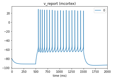
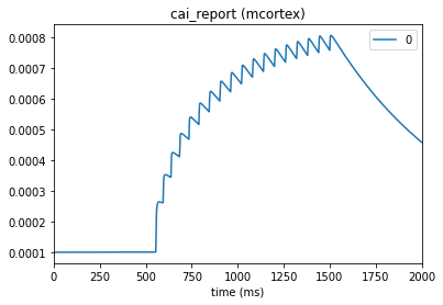
When setting up the environment and config file in section 2, “Setting up the simulator environment”, we specified cell_vars=['v', 'cai']. This indicates to the simulator to also record membrane potential and Ca2+ level. Other variables can also be specified when building the simulator environment as long as they are supported in NEURON.
[7]:
from bmtk.analyzer.compartment import plot_traces

_ = plot_traces(config_file='sim_ch01/config.json', node_ids=[0], report_name='v_report')
_ = plot_traces(config_file='sim_ch01/config.json', node_ids=[0], report_name='cai_report')
5. Additional information#
Changing run-time parameters#
By making changes to the config file, we can change the conditions and simulation parameters without having to rebuild the network, modify parameter files or change our run_bionet script. In fact we can iteratively run multiple simulations without any extra coding, only a text editor to change the JSON file.
The run section of the config.json file contains most of the parameters unique to the simulation:
{
  "run": {
    "dL": 20,
    "nsteps_block": 5000,
    "spike_threshold": -15,
    "tstop": 2000.0,
    "dt": 0.1
  }
}
tstop - Simulation runtime in milliseconds.
dt - Time steps of the simulation. Decreasing dt should increase accuracy of firing dynamics, but also increase the time it takes to complete.
spike_threshold - Used to determine when to count an action potential.
dL - Length of segments in a section. The number of segments will be forced to an odd number so the actual length may vary by one.
Through the conditions section we can adjust the simulation temperature (in degrees Celsius) and the initial membrane potential of the cells (in mV):
{
  "conditions": {
    "celsius": 34.0,
    "v_init": -80
  }
}
And lastly, the input section lets us control stimulus onto the network. There are a number of different options which will be explained in the following tutorials. But even with a simple current injection we can adjust the amplitude, delay and stimulation duration and measure the effect on the cell.
{
  "inputs": {
    "current_clamp": {
      "input_type": "current_clamp",
      "module": "IClamp",
      "node_set": "all",
      "amp": 0.120,
      "delay": 500.0,
      "duration": 1000.0
    }
  }
}
We can even add multiple injections:
{
  "inputs": {
    "cclamp1": {
      "input_type": "current_clamp",
      "module": "IClamp",
      "node_set": "all",
      "amp": 0.150,
      "delay": 0.0,
      "duration": 400.0
    },

    "cclamp2": {
      "input_type": "current_clamp",
      "module": "IClamp",
      "node_set": "all",
      "amp": 0.300,
      "delay": 500.0,
      "duration": 400.0
    },

    "cclamp3": {
      "input_type": "current_clamp",
      "module": "IClamp",
      "node_set": "all",
      "amp": 0.450,
      "delay": 1000.0,
      "duration": 400.0
    }
  }
}
Changing cell models#
When building the network we defined the cell model and morphology through the ‘dynamics_params’ and ‘morphology_file’ options. After building and saving the network, these values were saved in the node-types CSV file:
[8]:
import pandas as pd
pd.read_csv('sim_ch01/network/mcortex_node_types.csv', sep=' ')
[8]:
| node_type_id | model_template | morphology | model_processing | potential | model_type | dynamics_params | cell_name | |
|---|---|---|---|---|---|---|---|---|
| 0 | 100 | ctdb:Biophys1.hoc | Scnn1a_473845048_m.swc | aibs_perisomatic | exc | biophysical | 472363762_fit.json | Scnn1a_473845048 |
If we want to run the simulation on a different cell model, all we have to do is:
Download new json parameters and swc morphology files into the “components/biophysical_neuron_models” and “components/morphologies” folders
Open mcortex_node_types.csv in a text editor and update the ‘morphology_file’ and ‘params_file’ parameters accordingly.
In our simple one-cell example, it is likely faster to just rebuild the network. However the advantage of the use of the node types becomes clear once we start dealing with a larger network. For example we may have a network of hundreds of thousands of individual cells with tens of thousands of Scnn1a type cells. The process of adjusting/changing the Scnn1a parameter in the CSV file then starting another simulation takes only seconds, whereas rebuilding the entire network may take hours.
[ ]: