Running Network Simulations with BMTK#
In this section we will show how to use BMTK and SONATA to run simulation(s) on a brain network model.
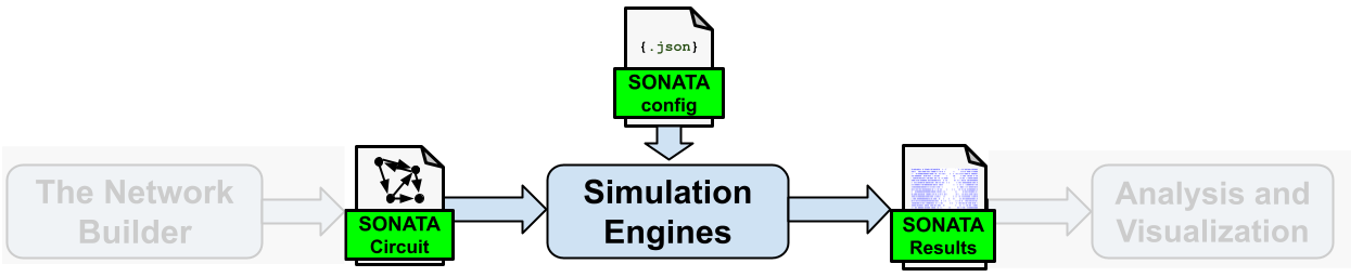
Unlike other neural simulation tools which will create and simulate a network in one script, BMTK workflow design is to split up these two parts of the process. So before we can run a simulation we must first obtain a network model (typically stored using the SONATA circuit format). We can either download an existing model, or alternatively use a tool like the BMTK Network Builder to create one from scratch.
Once we have our network to run simulations on, we typically need to complete the following steps:
Setup the enviornment. For most networks, this entails downloading or creating any auxiliary files required for network instantiation (morphology files, cell parameters, mod files, etc) and inputs (spikes, electrodes).
Setup the SONATA configuration file(s). We use a json based SONATA configuration file to instruct BMTK how to instiante a network (including location of circuits and any auxiliary files), run-time parameters, and what stimuli to use as input and what variables to record for our output. We can create a SONATA config file from scratch, or download and edit an existing one using a text editor.
Run the simulation(s). The majority of BMTK simulation can be fully defined in the SONATA config (although for advanced users BMTK allows extensive customization using Python). Thus we just need to execute a pre-generated python script with the above SONATA config file and let our simulation finish.
Once the simulation has completed, it will automatically generate and save the results as specified in the SONATA configuration file. Although BMTK can run network models of different levels-of-resolutions, and user can choose the appropriate underlying simulator library, e.g. Simulation Engine depending on the cell models. BMTK abstracts the interface to the simulators with SONATA files, so no matter if the network is run using NEURON, NEST, DiPDE, or any other engine; the expected inputs and outputs are the same format
The rest of this guide will go through each of the above steps in detail.
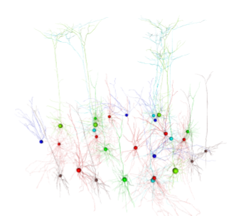
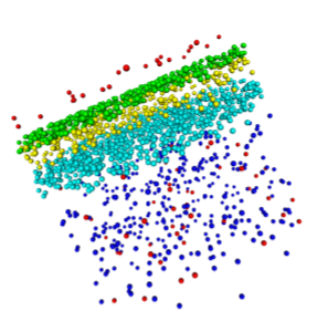
To help make the concepts for concrete we will also be referencing the example network simulation found here. This is a biophysically detailed network containing a 450 cells with a mixture of both multicompartment biophysically detailed neurons with parameters and morphologies download from the Allen Cell Types Database, surrounded by a ring of point integrate-and-fire neurons. For the main configuration, feedforward synaptic stimuli will emerge from virtual cells firing at a randomized rate.
1. Setting up the Environment#
First step is to download and/or create files necessary to instantiate network and execute the simulation. At miniumum, we require the SONATA circuit file(s), simulation configuration file, and a BMTK run script. In addition, we may also need the followings depending on the type of the model and simulation:
template files used to build the cell or synapse models (Hoc Templates, NeuroML, NESTML)
cell and synaptic dynamics attribute values,
cell morphologies (SWC, Neurolucdia),
simulation input and stimuli (spike-trains, current waveform, movie and auditory files),
NEURON .mod files.
We can put these files wherever we want as long as they are accessible during simulation execution. Although best practices is to put them inside a single directory with the following structure.
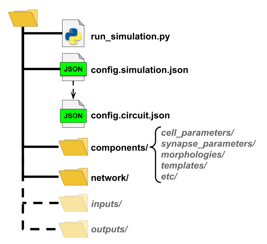
BMTK includes the create_environment tool that can help new users generate an environmental directory from scratch. Another option we recommend, especially if running simulations on an already existing model, is to download an existing simulation environment and make changes as necessary.
When creating the BioNet example we used the build_network.py python script to build and save the network model into the network/ subdirectory (see BMTK Builder Guide for more information on that process). With the network built, we used the following command to generate baseline strucutre plus config.simulation.json configuration and the run_bionet.py script used to execute the simulation:
$ python -m bmtk.utils.create_environment         \
                --config-file config.iclamp.json  \
                --overwrite                       \
                --network-dir network             \
                --output-dir output_iclamp        \
                --tstop 3000.0                    \
                --dt 0.1                          \
                --report-vars v                   \
                --iclamp 0.150,500,2000           \
                --compile-mechanisms              \
                bionet .
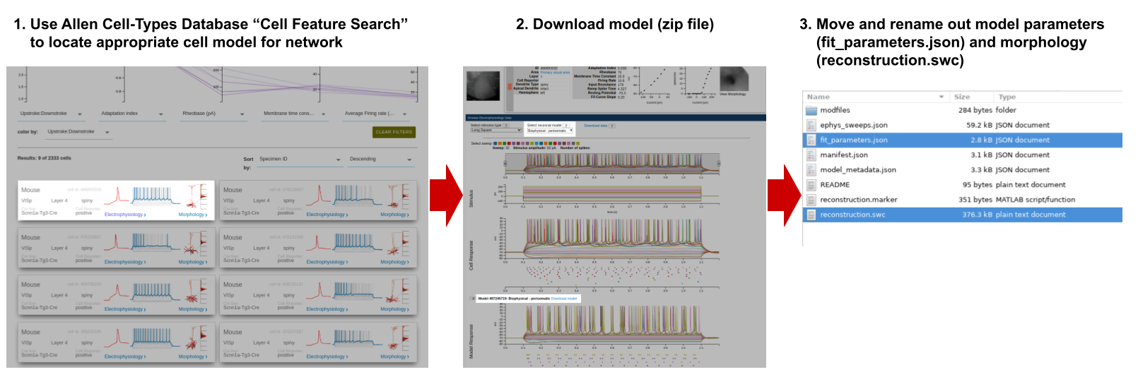
This script will create the components/ directory to place any auxiliary files for network instantiation, but unless explicity defined, the corresponding subdirectory will be empty. In particular our model’s various cell-types require SWC morphology and dynamics parameters files that can be downloaded from the Allen Cell Types Database, renamed and placed into their corresponding folders.
For simulation input our network will be stimulated by feed-forward pre-generated spike-trains that will be saved into the inputs/ folder using the create_inputs.py script
$ python create_inputs.py
2. Setting up Sonata Config file(s)#
The primary interface thorugh which most users will run a simulation is through the SONATA confiugration file(s). Each simulation will have its own json config file that can be opened and modified by any text editor, allowing users to readily adjust simulation, network, input, and output of any given simulation without requiring coding or having to learn the API for a specific simulator.
The config file is segmented into sections for the various aspects of running a full simulation. We will go into depth of each section below.
“run”#
The “run” section allows us to set run-time parameters for the simulation. At minimum, this includes the tstop parameter that determines the time step (in ms) when the simulation will stop. Other options, including tstart (time at start of simulation, ms) and dt (time step interval, ms), may or may not be optional or even used depending on the simulation.
The following attributes can be set for BMTK in the “run” section.
“run” simulation attributes
name
description
required
tstart
Start time of simulation in ms (default 0.0; not currently used in BMTK)
False
tstop
Stop time of simulation in ms
True
dt
The time step of a simulation; ms
True
dL
For networks with morphological models, is a global parameter used to indicate to the simulator the maximum length of each compartmental segment, in microns. If “dL” parameter is explicitly defined for a specific cell or cell-type, then BMTK will default to the more grainular option.
False
spike_threshold
For networks using conductance based model, is a global paramter to indicate the threshold in mV at which a cell undergoes an action potential. Will not apply to integrate-and-fire type models. Value will be overwritten for any cell or cell-type that explicity defines “spike_threshold” parameter in network attribute.
False
nsteps_block
Used by certain input/report modules to indicate time processing of timestep in blocks of every n time-steps. In particular for recording of spike-trains, membrane variables, or extraceullar potential; tells the simulation when to flush data out of memory and onto the disk.
False
The “run” section for our example simulation contains the following:
"run": {
  "tstop": 3000.0,
  "dt": 0.1,
  "dL": 20.0,
  "spike_threshold": -15,
  "nsteps_block": 5000
},
This will tell our simulation to run for 3,000 ms (3 seconds) with 0.1 ms timesteps, block process all the data every 5000 steps (eg. 500 ms). The “dL” makes sure that for morphologically detailed cells each branch segment is no more than 20 microns in length. And to record a spike when a cell reaches the threshold of -15.0 mV.
“inputs”#
The “inputs” section of the SONATA config file is used to specify stimli to apply to the network. It will contain one or more independent stimulus blocks of the format:
{
    "<BLOCK_NAME>": {
        "input_type": "<STIMULUS_TYPE>",
        "module": "<STIMULUS_FORMAT>",
        "node_set": "<NODES_SUBSET>",
        "param1": "<VAL1>",
        "param2": "<VAL2>",
        "paramN": "value"

    }
}
The <BLOCK_NAME> is the name of the stimulus block, users can choose whatever name they want to identify a specific stimulus.
input_type specifies the nature of the stimlulation, eg. if cell activity is being generated by synaptic events, current clamps, etc. The available options will depend on the resolution of the model and the type of cell models used. The options will depend on the input_type
module is used to indicate the format of the stimuli. For example, in trying to stimulate the network with virtual spiking activity file, the individual spike times may be stored in a SONATA spikes file, a NWB file, a CSV, etc.
node_set is a dictionary or reference used to select which cells to apply the current stimulus to.
Most stimuli will have one or more parameters options, depending on the input_type and module.
The following is a list of input types supported in BMTK. For further details about how to implement a given input in a simulation please see the corresponding documentation.
Available “input_type” stimuli
input_type
module
description
available
current_clamp
Directly injects current into one or more cells in the network. Shape of the stimulus may be a simple block, or user may specify more advanced current form using a csv, nwb, or hdf5 file.
BioNet, PointNet
spikes
Reads a table of spike train events into one or more virtual cells in the network.
BioNet, PointNet
voltage_clamp
SEClamp
Applys a voltage clamping block onto one or more cells.
BioNet
extracellular
Applies an extracellular potential to a selected set of cells in the network. Can replicate extracellular stimulation coming from an electrode (xstim) or pre-generated field (comsol).
BioNet
replay
replay
Allows users to “replay” the recurrent activity of a previously recorded simulation with a selected subset of cells and/or connections. Useful for looking at summative contributions in large networks.
BioNet, PointNet
syn_activity
Provides spontaneous firing of a select subset of recurrently connected synapses. Users may pre-specify firing times or let BMTK generate them randomly.
BioNet
movie
movie
Plays a movie (e.g. a numpy matrix file) onto the receptive field of a grid of neurons to mimic the visual response.
FilterNet
movie
Automatically generate a movie of one of a number of well-known experimental stimuli and use it to play onto the receptive field of a set of neurons.
FilterNet
The “inputs” section for our 400 cell example looks like the following:
"inputs": {
  "external_spikes": {
    "input_type": "spikes",
    "module": "sonata",
    "input_file": "./inputs/external_spikes.h5",
    "node_set": "external-cell"
  }
}
The “external_spikes” block tells BMTK that it will stimulate our network using SONATA spike-trains. The input spike trains were generated by running
$ python create_inputs.py
which will create a SONATA spike-trains file in inputs/external_spikes.h5. The node-set parameter, explained below, tells the module which cells we want to assign our spike-trains.
“components”#
The “components” section is used to indicate the paths to various auxiliary files required for instantiating our simulation; like morphology swc files, NEURON mod files, NESTML or NeuroML cell models.
The directories are defined using the format:
"components": {
    "<COMPONENT_TYPE>": "/path/to/components/dir/"
}
Recognized “components” directories
name
description
utilized by
biophysical_neuron_models_dir
Directory containing files for instantiation of biophysically detailed models. Typically containing json cell model files downloaded from the Allen Cell-Types Database.
dynamics_params
point_neuron_models_dir
Directory containing files for instantiation of point-neuron models. Typically json parameter files, or model files downloaded from the Allen Cell-Types Database to instantiate optimized “GLIF” models.
dynamics_params
filters_dir
Directory containing parameter files for instantiating models used by FilterNet.
dynamics_params
morphologies_dir
Directory containing any morphological reconstruction files (ex. swc, neurolucdia).
morphology
synpatic_models_dir
Directory containing files for specific synaptic parameters.
dynamics_params
mechanisms_dir
Directory containing any morphological reconstruction files (ex. swc, neurolucdia)
templates_dir
Contains NEURON Hoc template files or NeuroML cell or synapse models.
model_template
For our example network,
"components": {
  "morphologies_dir": "$COMPONENT_DIR/morphologies",
  "synaptic_models_dir": "$COMPONENT_DIR/synaptic_models",
  "mechanisms_dir":"$COMPONENT_DIR/mechanisms",
  "biophysical_neuron_models_dir": "$COMPONENT_DIR/biophysical_neuron_templates/nml",
  "point_neuron_models_dir": "$COMPONENT_DIR/point_neuron_templates"
}
“output” and “reports”#
The “outputs” section defines where and how to save simulation results. The most important element is the output_dir attribute that defines the default location of the files generated during the simulation. The spikes_file attribute defines the name of the file (relative to the output_dir path) in which BMTK store any non-virtual spikes generated during the simulation in the SONATA hdf5 format.
“output” attributes
name
description
default value
output_dir
Path of output folder where simulation results and temp files will be saved in. BMTK will create the folder if it does not already exists. If the value is not an absolute path, then will assume to be relative to location where BMTK simulation is being executed (i.e. os.getcwd())
.
overwrite_output_dir
If set to True then BMTK will overwrite any previous output files stored in output_dir. If set to False and files exists before run time then BMTK may throw an error and exit simulation.
True
log_file
Name of the file to which BMTK messages will be written. If the file name has a relative path, file will be saved underneath output_dir. If the value is set to false or none then no log file will be created during simulation.
none
log_level
Level of logging information that will be included during simulation (DEBUG, INFO, WARNING, ERROR).
DEBUG
log_format
The format string for how BMTK will save log messages. It uses the LogRecord attributes options set by python’s logging module.
%(asctime)s [%(levelname)s] %(message)s
log_to_console
If true then will also log output to default standard output (stdout), if false then will disable stdout logging. Note: if both log_to_console and log_file are set to false then BMTK will not log any simulation messages (simulation will still run and produce results).
true
quiet_simulator
Can be set true to turn off any messages generated by the underlying simulator (NEURON, NEST, DiPDE)
false.
spikes_file
Location of the hdf5 file in which spikes will be saved. If the location is a relative path, file will be saved under the output_dir directory. If set to none, no SONATA spikes file will be created during simulation.
none
spikes_file_csv
Location of the space separated csv file in which spikes will be saved. If the location is a relative path, file will be saved under the output_dir directory. If set to none, no csv spikes file will be created during simulation.
none
sort_by
none
By default BMTK will save non-virtual spike-trains of the simulation. BMTK is also capable of saving many other cell, synapse, and even network wide parameters and attributes during a simulation, like membrane potential, Calcium concentration, or local field potentials. To instruct BMTK to record a extra parameter we must add one or more blocks to the “reports” subsection (at the same level as “output”, not within) to config, which will have the following format:
"reports": {
    "<BLOCK_NAME>": {
        "module": "<REPORT_TYPE>",
        "input_type": "<REPORT_VAR>",
        "cells": "<NODES_SUBSET>",
        "file_name": "<FILE_NAME>",
        "param1": "<VAL1>",
        "param2": "<VAL1>"

    }
}
The <BLOCK_NAME> is a user-given identifier for a different report, each different block assumed to be independent of each other.
module indicates the report type and nature.
variable_name indicates the variable in the simulation being recorded.
cells is a node-set that are recorded.
file_name is an optional path for where module will save output. If path is relative, it will assume to be saved under the output_dir path specified in “output” block. If not specified, BMTK will attempt to infer the correct path (usually under output_dir/<BLOCK_NAME>.h5
Different modules may also have different required/optional parameters. The following is a list of BMTK supported “report” modules:
Available “report” modules
module
description
available
membrane_report
Used to record a time course of a cell such as membrane voltage or calcium concentration
BioNet, PointNet
syn_report
Used to record a time course of variables for the synapses of a given set of cells
BioNet, PointNet
syn_weight
Record of synaptic weight changes for a given set of cells.
BioNet, PointNet
extracellular
Used to record a time course of extracellular field potential for a given set of electrodes
BioNet
For our 400 cell example we will want to have all the output generated by BMTK be written to the output/ folder, including the log which will be written to output/log.txt. It will also create two spike-train files on the (non-virtual) cells recorded from all cells during the simulation, output/spikes.h5 and output/spikes.csv. Both files will contain the exact same data; one will be stored in a SONATA hdf5 file and another in a space-separated csv file.
"output":{
  "output_dir": "./output",
  "overwrite_output_dir": true,
  "log_file": "log.txt",
  "spikes_file": "spikes.h5",
  "spikes_file_csv": "spikes.csv"
}
Besides recording spikes, we also want to record the local field potentials of all cells plus the membrane voltage traces for a selected set of cells, which we do in the following two blocks in the “reports” section, respectively.
"reports": {
  "vm_report": {
    "cells": "scnn1a-bio-cells",
    "variable_name": "v",
    "module": "membrane_report",
    "file_name": "vm_report.h5",
    "sections": "all"
  },

  "ecp": {
    "cells": "biophysical-cells",
    "variable_name": "v",
    "module": "extracellular",
    "electrode_positions": "./components/recXelectrodes/linear_electrode.csv",
    "file_name": "ecp.h5",
    "electrode_channels": "all",
    "contributions_dir": "ecp_contributions"
  }
}
The “vm_report” block will instruct BMTK to record membrane traces from all “scnn1a” type cells and save them in the SONATA formated output/vm_report.h5 file. If you wanted to record membrane potential from other cell types you have the option of either modifying the “vm_report” block to save the membrane traces of other cells to the same output/vm_report.h5 file. Or, alternatively, create another block that will independently save a different set of cell voltage traces into a different file.
The “ecp” block will record the local field potential (LFP) and save it to the file output/ecp.h5.
Note that recording LFP and membrane voltages at every time step can signficantly increase simulation time and their resulting output files can become very large. So if you only care about spikes and firing rates then you can either remove these “report” blocks from the configuration file, or set attribute “enabled”: false
“networks”#
The “networks” section contains paths to any SONATA network files, cells and connections, used during our simulation. By default it is divided into two subsections: one containing any nodes (cells) files used during the simulation, and the other containing and edges (synapses) files used, with the following format:
"networks": {
    "nodes": [
        {
            "nodes_file": "</path/to/nodes.h5>",
            "node_types_file": "</path/to/node_types.h5>"
        }
    ],
    "edges": [
        {
            "edges_file": "</path/to/edges.h5>",
            "edge_types_file": "</path/to/edge_types.h5>"
        }
    ]
}
BMTK will go through each of the nodes.h5 and edges.h5 files and import all nodes and edges found, respectively. If a file contains both nodes and edges then the file must be added to both the “nodes” list and the “edges” list to include the total network.
The main set of cells we want to simulate our example is saved under the file name, intenral_nodes.h5, with the recurrent connections between the cells are saved in the file, internal_internal_edges.h5. If we wanted to run a simulation with these cells with either spontaneous input or some form of clamp we specify them using the “inputs” section; then we could do the following in our configuration file:
"networks": {
  "nodes": [
    {
      "nodes_file": "$NETWORK_DIR/internal_nodes.h5",
      "node_types_file": "$NETWORK_DIR/internal_node_types.csv"
    }
  ],

  "edges": [
    {
      "edges_file": "$NETWORK_DIR/internal_internal_edges.h5",
      "edge_types_file": "$NETWORK_DIR/internal_internal_edge_types.csv"
    }
  ]
}
However, in this example, we explicity want to synaptically stimulate the “internal”, which we can do using a separate population of virtual cells we that name “external”. The external_nodes.h5 contain a population of virtual cells while the external_internal_edges.h5 file is used to synaptically connect the “external” virtual cells to our “internal” cells.
"networks": {
  "nodes": [
    {
      "nodes_file": "$NETWORK_DIR/internal_nodes.h5",
      "node_types_file": "$NETWORK_DIR/internal_node_types.csv"
    },
    {
      "nodes_file": "$NETWORK_DIR/external_nodes.h5",
      "node_types_file": "$NETWORK_DIR/external_node_types.csv"
    }
  ],

  "edges": [
    {
      "edges_file": "$NETWORK_DIR/internal_internal_edges.h5",
      "edge_types_file": "$NETWORK_DIR/internal_internal_edge_types.csv"
    },
    {
      "edges_file": "$NETWORK_DIR/external_internal_edges.h5",
      "edge_types_file": "$NETWORK_DIR/external_internal_edge_types.csv"
    }
  ]
}
When BMTK runs, it will create both the “internal” and “external” population of cells and generate all external –> internal and internal <–> internal synaptic connections. The “inputs” section of the configuration will assign firing patterns to the “external” cells, creating stimuli to our network.
“node_sets”#
During a simulation we often want to apply an input or report to only a specific subset of cells. For example, we may want voltage traces from only pyramidal cells. We can do this by using the “node_sets” subsection, and creating subsets of our network model that can be referenced in the rest of the config:
"node_sets": {
  "<SET-NAME-1>": {
    "population": "cortical",
    "node_id": [100, 101, 103, 104]
  },
  "<SET-NAME-2>": {
    "model_type": "biophysical",
    "cell_description": "pyramidal",
    "cell_location": "L23"
  }
},

"reports": {
  "vm_report": {
    "module": "membrane_report",
    "variable_name": "v",
    "cells": "<SET-NAME-1>",
    // ...
  },

"inputs": {
  "iclamp_stimulus": {
        "input_type": "current_clamp",
        "module": "ICLAMP",
        "node_set": "<SET-NAME-2>",
        // ...
      }
    }
For <SET-NAME-1>, the node-set will tell BMTK to record from only those cells with specified node ids. If you don’t know the exact node_ids, or if there are too many to feasibly write down, you can filter by cell attributes. In <SET-NAME-2> we are directing BMTK to apply current clamp to all biophysical pyramidal cells found in L23.
Users also have the option of embedding the “node-set” query parameters directly. The below example will apply inputs to the exact same subset of cells as done in the above.
"inputs": {
  "iclamp_stimulus": {
        "input_type": "current_clamp",
        "module": "ICLAMP",
        "node_set": {
          "model_type": "biophysical",
          "cell_description": "pyramidal",
          "cell_location": "L23"
        },
        // ...
      }
    }
For our 400 cell example we need 3 different node-sets
"node_sets": {
  "external-cells": {
    "population": "external",
    "model_type": "virtual"
  },
  "bio-cells": {
    "model_type": "biophysical"
  }
  "scnn1a-bio-cells": {
    "population": "internal",
    "model_name": "scnn1a"
  }

}
The external-cells set contains all cells in our “external” population of virtual cells to which spike trains are assigned in the “inputs” section.
The bio-cells set is required by “ecp” recording block. Our model contains both morpholigcally detailed and point-neuron models, but only the former can be used to record the local field potential. Passing “node_set”: “bio-cells” to the ecp module will make sure the module doesn’t crash trying to record from cell models that don’t produce extracellular potential.
The scnn1a-bio-cells set is used by the “vm_report” recording block so that it knows only to record voltage traces that have their “model_name” attribute set to value “scnn1a”. Although we could record “v” varaible from all cells, doing so would increase simulation time and generate a lot of extra data we don’t need.
“manifest” [OPTIONAL]#
The “manifest” section lets users define variables and special directives to be used throughout the rest of the configuration file. SONATA uses the standard “$” posix prefix for differentiating a constant versus a varaible.
For example, we use the manifest in the following manner to create custom variable “$NETWORK_DIR”
"manifest": {
   "$NETWORK_DIR": "$/path/to/my/models/network/"
},

"networks": {
   "nodes": [
     {
       "nodes_file": "$NETWORK_DIR/network1_nodes.h5",
       "node_types_file": "$NETWORK_DIR/network1_types.csv"
     },
     {
       "nodes_file": "$NETWORK_DIR/network2_nodes.h5",
       "node_types_file": "$NETWORK_DIR/network2_types.csv"
     }
   ]
 }
This way if we need to change the location of our network files or copy it to a new drive we can simply update the manifest in one single place.
Splitting the config [OPTIONAL]#
Sometimes it is convenient to think of the SONATA configuration as two parts; the simulation part with the “run”, “inputs”, and “reports” sections, and the network part with the “networks” and “components” sections. BMTK allows configuration file to be split, first by splitting into respective json files, for example called ./path/to/config.simulation.json and ./path/to/config.network.json (you can use whatever name and path). Then to import these two sections into one file just use the following:
{
  "simulation": "./path/to/config.simulation.json",
  "network": "./path/to/config.network.json"
}
And when BMTK runs it will locate and combine both configuration into one json dictionary.
If you want to reduce the number of files, you can also import a separate “network” config into a “simulation” config (or vice-versa).
{
  "run": {
    // ...
  },
  "inputs": {
    // ...
  },
  "reports": {
    //...
  },

  "network": "./path/to/config.network.json"
}
This can be useful if you have multiple simulations on the same network with different input regimens. It ensures that each simulation config use the same model. And if you have to update the model and/or component paths, you only need to do so once.
3. Run the Simulation#
Now we have all the files we need to instantiate the model, along with a configuration that specifies the run-time, inputs, and reporting conditions of our simulation. We can go ahead and execute the simulation using the following command:
$ python run_simulation.py config.simulation.json
If you have a machine or cluster with multiple cores, you can instruct BMTK to parallelize the simulation. The only change the user will have to make is to change the way python is called to comply with your setup.
$ mpirun -np N python run_simulation.py config.simulation.json
where N is the number of processes you run simultaneously. The simulation can also be executed inside Jupyter notebook/lab if prefered. Just copy the contents of the run_script (see below) into the cell and execute as you would a normal notebook.
There are numerious other options for ways to execute BMTK; including:
Docker Image: The BMTK Docker image allows users to run BMTK through a virtual machine containing a pre-generated environment with BMTK and all dependencies installed. You can use docker run command to run a simulation on your machine, or even spin up a Jupyter lab server (that will include BMTK tutorials and examples).
See Using Docker with BMTK guide for more information.
Neuroscience Gateway (NSG): Running BMTK on the Neuroscience Gateway (NSG)
singularity
Run script#
For the majority of use-cases, users will not need to do any programming as most simulation options can be set using the SONATA simulation configuration file. But BMTK does allow users to insert customized code and data into any simulation. To do so, you will need to modify the default run_simulation.py script used to run a simulation.
If you want to modify the way BMTK executes, and/or run a BMTK simulation from a Jupyter cell or within another piece of code, use the code within the run() function . Note: There are slight differences in the run script depending on the underlying “simulation engine” used, although they all follow the same structure.
 1import sys
 2from bmtk.simulator import bionet
 3
 4def run(config_path):
 5    config = bionet.Config.from_json(config_path)
 6    config.build_env()
 7
 8    graph = bionet.BioNetwork.from_config(config)
 9    sim = bionet.BioSimulator.from_config(config, network=graph)
10    sim.run()
11
12    bionet.nrn.quit_execution()
13
14if __name__ == '__main__':
15    run(sys.argv[-1])
description of run() function by lines #
Loads in the config.simulation.json file into python a dictionary-like object, resolving any variables, paths, and directives.
Sets up logging and creates and validates any directories/files to be used for recording simulation output.
Initializes the network using the SONATA configuration file’s “networks” section.
Initializes the simulation.
Runs the simulation.
Because BioNet runs within a NEURON console, we must explicity exit() it.
 1import sys
 2from bmtk.simulator import pointnet
 3
 4def run(config_path):
 5    config = pointnet.Config.from_json(config_path)
 6    config.build_env()
 7
 8    network = pointnet.PointNetwork.from_config(config)
 9    sim = pointnet.PointSimulator.from_config(config, network)
10    sim.run()
11
12if __name__ == '__main__':
13    run(sys.argv[-1])
description of run() function by lines #
Loads in the config.simulation.json file into python a dictionary-like object, resolving any variables, paths, and directives.
Sets up logging and creates and validates any directories/files to be used for recording simulation output.
Initializes the network using the SONATA configuration file’s “networks” section.
Initializes the simulation.
Runs the simulation.
 1import sys
 2from bmtk.simulator import filternet
 3
 4def run(config_path):
 5    config = filternet.Config.from_json(config_path)
 6    config.build_env()
 7
 8    net = filternet.FilterNetwork.from_config(config)
 9    sim = filternet.FilterSimulator.from_config(config, net)
10    sim.run()
11
12if __name__ == '__main__':
13    run(sys.argv[-1])
description of run() function by lines #
Loads in the config.simulation.json file into python a dictionary-like object, resolving any variables, paths, and directives.
Sets up logging and creates and validates any directories/files to be used for recording simulation output.
Initializes the network using the SONATA configuration file’s “networks” section.
Initializes the simulation.
Runs the simulation.
 1import sys
 2from bmtk.simulator import popnet
 3
 4def run(config_path):
 5    configure = popnet.config.from_json(config_path)
 6    configure.build_env()
 7
 8    network = popnet.PopNetwork.from_config(configure)
 9    sim = popnet.PopSimulator.from_config(configure, network)
10    sim.run()
11
12if __name__ == '__main__':
13    run(sys.argv[-1])
description of run() function by lines #
Loads in the config.simulation.json file into python a dictionary-like object, resolving any variables, paths, and directives.
Sets up logging and creates and validates any directories/files to be used for recording simulation output.
Initializes the network using the SONATA configuration file’s “networks” section.
Initializes the simulation.
Runs the simulation.
Simulation results#
Depending on the complexity of the model and inputs and reports, a simulation may take seconds to days to complete. By default, BMTK will save any results and “reports” as set up in the SONATA config. Once completed and results are saved, we can analyze our results, which we go into further details in the next section of the user guide.
We can run our 400 cell network simulation using the run_simulation.py script in our working directory.
The simplest way to run the simulation in a command line using a single core.
$ python run_simulation.py config.simulation.json
If you have MPI (Message Passing Interface) installed on you machine, use the following to split the simulation up between N cores (replace N with the number of cores/ranks).
$ mpirun -np N nrniv -mpi -python run_simulation.py config.simulation.json
To run the simulation inside a Jupyter notebook, add the following lines to a cell and execute:
from bmtk.simulator import bionet
config = bionet.Config.from_json("config.simulation.json")
config.build_env()
graph = bionet.BioNetwork.from_config(config)
sim = bionet.BioSimulator.from_config(config, network=graph)
sim.run()
If you have a docker client installed on your machine, you can use the following to execute the simulation:
$ docker run alleninstitute/bmtk -v local/path:/home/shared/workspace python run_simulation.py config.simulation.json
When it starts, the first thing it will do is to create (or overwrite) the output/ folder along with output/log.txt log file that keeps track of the progress of the simulation. Although this network is small enough to run on any modern computer or laptop, it will still take anywhere between 5 to 30 minutes to complete, depending on the hardware.
Once completed, it will create the following files:
output/spikes.h5 and output/spikes.csv contain spike trains for all non-virtual cells. (Both files have the same data but in different file formats).
output/vm_reports.h5 contains membrane traces of selected cells in SONATA formated hdf5 file.
ouput/ecp.h5 contains local field potential (LFP) recordings from all the biophysically detailed cells, as recorded from simulated electrodes, and saved in the SONATA hdf5 format.
Simulation Engines#
As mentioned before, BMTK is capable of simulating a wide variety of different network models across multiple levels of cell resolutions. To do this, BMTK utilizes different backend simulator libraries, or “Simulation Engines”, depending on the nature of the model (ie. compartmental models, point models, filter models, rates based models, etc).
BMTK standardizes and abstracts the simulation process so that users can easily switch between model types without having to learn a whole new API. However, there are still important differences between the varying Simulation Engines. Some may excpect certain parameters and attributes (e.g. compartmental models will expect cells to have a defined morphology). Similarily, some may contain extra features and capabilities.
To learn more about the requirements and capabilities for the model(s) of your interest, please refer to the user guides of the corresponding simulation engine:
BioNet - Multicompartment Biophysicaly Detailed Simulation
BioNet utilizes the NEURON simulator to allow simulation of multicompartment cell models. It can incorporate cells’ full morphology into a model and a simulation, allowing you to simulate aspects including ion flow, membrane properties, and synaptic location and density.
PointNet - point-neuron based models
PointNet utlizes the NEST simulator for simulation of networks of point-neuron models, including Allen’s GLIF models, Izhikevich models, Hodgkin-Huxley, and many more. Most PointNet network models run faster with less overhead than BioNet and is a good starting point.
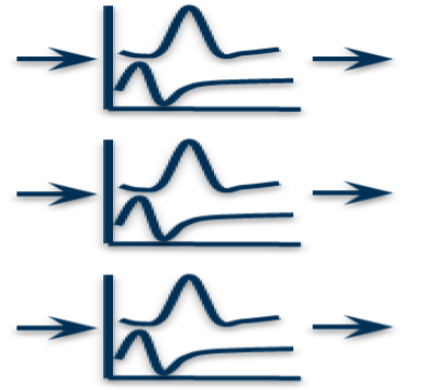
FilterNet - Receptive Field Filter Models
FilterNet allows users to play visual or auditory stimuli onto a linear-nonlinear filter model to generate realistic firing rates and spike trains based on the spatio-temporal properties of the stimuli. The results of which can be used by BioNet and PointNet as realistic stimuli.
PopNet - Population Wide Firing Rates Models
PopNet - Use’s Allen’s DiPDE solver to look at population level firing rate dyanmics.

Additional Resources and Guides#
Exectuion and Run Options#
The following guides and tutorials for setting up and running simulations across a wide variety of different computing environments.
Guides, tips and tricks for running bmtk using high-performance computing (HPC) resources with Message Passing Interface (MPI). Including tips for installing MPI, running on slurm, and using singularity container.
The Neuroscience Gateway is a tool for neuroscientists to access HPC resources for free. Guide shows how to use BMTK with the NSG web and API interface to build networks and run large simulations.
Comming Soon.
How to setup and run BMTK using pre-built applications and images; including with Docker, AppImage, and Snap.
How to run multiple simulations in parallel and/or serial; including grid searching, evolutionary, and gradient search methods for optimizing network and simulations.
Inputs for Simulations#
BMTK supports using a wide variety of inputs and stimuli when running a simulation. Please see the following guides for built-in “inputs” types and how to use them in your simulations.
Apply an excitatory or inhibitory current clamp to selected cells.
Create multiple square-wave stimulus blocks.
Using files and/or functions to create more complex current patterns.
How to choose locations along a cell’s morphology (BioNet).
Apply a voltage clamp to selected cells.
Input in the form of a square-block, or more complex patterns using files or functions.
How to select location to apply clamp (BioNet).
How to create you’re own pregenerated spike-train files using SONATA, CSV, or NWB files.
Write your own python function to dynamically generate input spike-trains before or during simulation.
Use NWB 2.0 files to insert experimental spike-sorted recordings into a simulation.
How to query and map NWB units onto simulation cells.
How to select events only from specific epochs, trials or intervals.
Use DANDI to automatically query and select experiments from multiple labs and experiments.
Use Allen Cell-Types intracullar experimental stimuli (sweep) for a simulation.
Use activity of previous recurrent recordings for input to simulation.
Allows you to capture and separate out network activity not generated by external stimulus.
Can also select subpopulations of cells and synapses to segment subnetwork and motif activity within a larger network.
Produce an extracellular field with an extracullar electrode or mesh.
How to set channel locations and extracellular resistance.
Use a constant field, sinusoidal wave, or your own custom voltage function.
How to use COMSOL physical simulator to stimulate with complex field dynamics.
Have synapses activiate without external pre-synaptic activity.
Can fire at regular, random, or pre-generated periods.
Choose cells based on pre, post, and/or connectivity attributes.
How to generate custom movies for a FilterNet stimulus.
Static Images and slide-shows.
Drifting Gratings.
Full-Field Flashes.
Looming movie.
Gaussian noise.
Reports#
Users can choose variables to record using the “reports” section. See following guides for further information to implement such output.
Record spikes from a selected subset of cells.
Saving to SONATA, CSV, and NWB 2.0 formats.
Sorting, indexing, and compression options.
Recording of membrane voltage, calcium concentration, and other ions/variables.
Selecting subsets of cells to record from.
Selecting morphological areas of cells to record from (BioNet).
Record weight changes in STP and STDP synapses.
Recording synaptic variables over the course of a simulation.
Get the original firing rate dynamics in response to visual or auditory stimuli in FilterNet.
Recording single and group cell contribution to a extracellular electrode or mesh.
Setting extracellular resistance.
Calculating Current Source Density.
Advanced Features#
Importing NEURON HOC template cell models.
Overwriting and appending to default cell model parameters and mechanisms.
Writing custom cell models in Python.
Importing customized channels and ion mechanisms into existing models.
Using Built-in NEST cell models.
Overridding cell model instantiation.
Custom cell models with NESTML