PointNet#
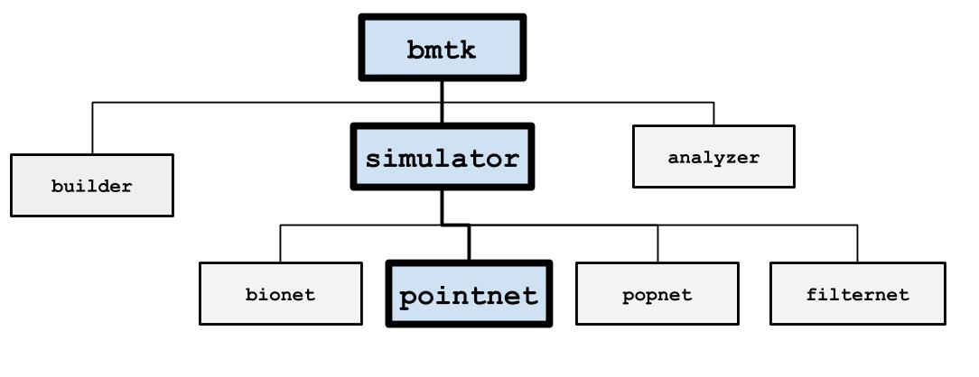
PointNet is a simulation engine that utilizes NEST to run large-scale point neuron network models. Features include:
Ability to run the same simulation on a single core or in parallel with no extra programming required
Support for any spiking neuron model available in NEST or with user contributed modules
Recording of neuron spike times and multi-meter variables in the optimized SONATA data format
To build a network in PointNet, please see the Network Builder overview.
For an example tutorial, please see Tutorial 5: Point-Neuron Network Models.
For an example network with 12,500 randomly connected excitatory and inhibitory point neurons, please see the BMTK github.
Inputs#
Inputs can be specified in the “inputs” sections of the simulation config, following the rules specified in the SONATA Data format.
Spike-Trains#
Cells with model_type value virtual are equivalent to NEST’s spike_generator model which plays a pre-recorded series of spikes throughout the simulation. You may use either a SONATA spike-train file, an NWB file, or a space-separated csv file with columns node_id, population, and timestamps. Examples of how to create your own spike-train files can be found here.
{
    "LGN_spikes": {
        "input_type": "spikes",
        "module": "sonata",
        "input_file": "./inputs/lgn_spikes.h5",
        "node_set": {"population": "lgn"}
    }
}
module: either sonata, hdf5, csv, or nwb: depending on the format of the spikes file
node_set: used to filter which cells will receive the inputs
input_file: a path to a file that contain spike-trains for one or more nodes. As a special case, a list of files can be provided to run multiple simulations with a single configuration file. See below for more information.
Extracelluar ElectroPhysiology (ECEPhys) Probe Data (NWB 2.0) Spikes#
An increasing number of public ECEPhys electrode experimental data are available in the NWB format, such as the Allen Visual Coding - Neuropixels dataset or the many datasets available on DANDI. While it is possible to manually convert this data into SONATA spike-trains to encorpate into your simulations, the ecephys_probe spikes module can do this automatically; fetching spikes from ECEPhys units and converting them to virtual cells for network input into your model.
For example, using a session NWB downloaded using the AllenSDK, the below example wil randomly map “LGd” cells from the session onto our “LGN” population, and filter out only spikes that occur between 10.0 and 12.0 seconds:
{
  "inputs": {
    "LGN_spikes": {
      "input_type": "spikes",
      "module": "ecephys_probe",
      "input_file": "./session_715093703.nwb",
      "node_set": {"population": "LGN"},
      "mapping": "sample_with_replacement",
      "units": {
        "location": "LGd"
      },
      "interval": [10000.0, 12000.0]
    }
  }
}
See the documentation for more information and advanced features.
Current Clamps#
Users may apply one step current clamp on multiple nodes, or multiple current injections to a single node.
{
    "current_clamp_1": {
        "input_type": "current_clamp",
        "module": "IClamp",
        "node_set": "biophys_cells",
        "amp": 0.1500,
        "delay": 500.0,
        "duration": 500.0
    }
}
See documentation for more details on using current clamp inputs.
Outputs#
Spikes#
By default all non-virtual cells in the circuit will have all their spikes recorded as if from the soma.
Membrane and Intracellular Variables#
Used to record the time trace of specific cell variables, usually the membrane potential (v). This is equivalent to NEST’s multimeter object.
{
    "membrane_potential": {
        "module": "multimeter_report",
        "cells": {"population": "V1"},
        "variable_name": "V_m"
        "file_name": "cai_traces.h5"
    }
}
module: either multimeter_report or membrane_report, which are interchangeable
variable_name: name of the variable being recorded; it will depend on the NEST cell model
cells: a node_set defines what cells to record
- file_name: name of the data file, under the “output_dir”. If not specified the the report title
will be used, i.e. “membrane_potential.h5”
Recording Synaptic Weights#
This module can be used to record the synaptic weight changes throughout the simulation lifetime. This tool is useful for measuring changes in plastic synapse models like “stdp_synapse” or “tsodyks_synapses” (can also be used for static synapses though values will never change). To create a recorder, add the following section to the “reports” section in the simulation config json:
{
    "reports": {
        "<name>": {
            "module": "weight_recorder",
            "nest_model": "<original-nest-model>",
            "model_template": "<recorder-name>",
            "file_name": "<file-name>.csv"
        }
    }
}
which will create a special synapse model called “<recorder-name>”, which is just a version of <original-nest-model> that will save a trace of the synaptic changes to the csv file output/<file-name>.csv. Just set the model_template property value to “<recorder-name>” in the edge-types file.
For example, to record the changes to a subset of the stdp_synapse type NEST models, add the following to the configuration:
{
    "reports": {
        "weight_recorder_stdp_1": {
            "module": "weight_recorder",
            "nest_model": "stdp_synapse",
            "model_template": "stdp_synapse_recorder",
            "file_name": "stdp_weights.csv",
        }
    }
}
Then make the following changes to the edge_types.csv file
edge_type_id |
model_template |
dynamics_params |
… |
|---|---|---|---|
100 |
stdp_synapse_recorder |
stdp_params.json |
… |
Running multiple simulations with a single config file#
PointNet supports running multiple simulations using a single configuration file. This file can include multiple inputs and outputs. This feature eliminates the need to create separate configuration files for each input/output file, and it allows similar simulations to run without the overhead of rebuilding the network each time. An example configuration file demonstrating this feature is located at ‘examples/point_450glifs/config.multiplesimulation.json’. Currently, this feature is only available with the sonata spikes input type, not with the current clamp, NWB, and spontaneous noise input types.
To use this feature, you must maintain a consistent structure in the ‘run’ section for ‘tstop’ (or equivalently, ‘duration’), in the ‘input’ section for ‘input_file’, and in the ‘output’ section for ‘output_file’. You can still have multiple input and output items, but their shape must be consistent.
If ‘tstop’ is provided as a list, its length determines the number of simulations to run. If ‘output_file’ is shorter than ‘tstop’, an error will occur. Similarly, if ‘input_file’ is shorter than ‘tstop’, a warning will be issued, and some simulations toward the end may not receive corresponding inputs.
The NEST state is not reset between simulations. Each sequential simulation inherits properties (such as membrane voltages and synaptic inputs) from the previous run. Also, the timestamps stored in the output files are not reset. For example, if the first simulation lasts 3000 ms, the timestamps in the second output file will begin at 3000 ms.
Although there is no method to force-reset the network (see nest/nest-simulator#1618), you can introduce an interval between simulations to allow neurons to return to their resting state. The simplest approach is to set ‘tstop’ longer than the stimulus period. For example, if your stimulus lasts 3000 ms, setting ‘tstop’ to 3500 ms will provide a 500 ms blank period at the end of the simulation, giving neurons time to go back to resting state before the next simulation.
Note that this implementation sets the onset of stimuli, but not their offset. If a stimulation file is longer than ‘tstop’, its input will continue into subsequent simulations.
Combining these features, you can, for example, use a single background Poisson spike file with an extended duration alongside multiple short LGN input files with different patterns, all in one configuration file. Also, other input types (e.g. current clamp) can be used if the stimulus time refers to the overall simulation time.
When ‘tstop’ is the same for all simulations, you can also use the ‘n_runs’ option in the ‘run’ section. Internally, this creates a list for ‘tstop’ where each entry has the same value, repeated ‘n_runs’ times.
Here are examples of valid options:
{
    "run": {
        "tstop": [1500, 2500, 3500],
    },
    "inputs": {
        "LGN_spikes": {
            "input_type": "spikes",
            "module": "sonata",
            "input_file": [
                "./inputs/lgn_spikes0.h5",
                "./inputs/lgn_spikes1.h5",
                "./inputs/lgn_spikes2.h5"
            ],
            "node_set": {"population": "lgn"}
        }
    },
    "output": {
        "log_file": "log.txt",
        "spikes_file": [
            "spikes0.h5",
            "spikes1.h5",
            "spikes2.h5"
        ],
        "output_dir": "./output"
    }
}
In this example, 3 simulations will be run. Each simulation will have a different duration, and will be stored separately. The assumption here is that the LGN input has durations that corresponds to the simulation durations.
{
    "run": {
        "duration": 3000,
        "n_runs": 2
    },
    "inputs": {
        "LGN_spikes": {
            "input_type": "spikes",
            "module": "sonata",
            "input_file": [
                "./inputs/lgn_spikes0.h5",
                "./inputs/lgn_spikes1.h5"
            ],
            "node_set": {"population": "lgn"}
        },
        "BKG_spikes": {
            "input_type": "spikes",
            "module": "sonata",
            "input_file": [
                "./inputs/bkg_spikes.h5"
            ],
            "node_set": {"population": "bkg"}
        }
    },
    "outputs": {
        "log_file": "log.txt",
        "spikes_file": [
            "spikes0.h5",
            "spikes1.h5"
        ],
        "spikes_file_csv": [
            "spikes0.csv",
            "spikes1.csv"
        ],
        "output_dir": "./output"
    }
}
In this example, 2 simulations with the same duration will be run. The LGN input will be distinct for the two simulations, but the BKG spikes is a single file. If the BKG spikes file has sufficiently long duration (6 s in this case), it will continue into the second simulation. The output files can be multiple types, each with a corresponding list of filenames.