Analyzing the Results#
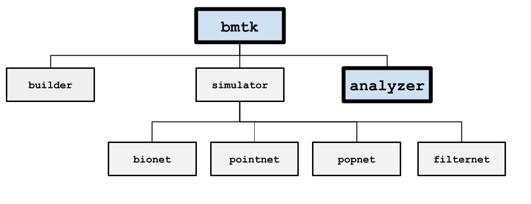
When a simulation has been completed, BMTK will save the results to the output folder. It is possible to have BMTK read and analyze the results before the simulation has exited but is usually not required. The type of results saved during the simulation is determined by the “reports” section of the simulation config. But most commonly it is a spikes-train file, a cell-variable report, an extracellular potential recording, and ,in the case of PopNet, a report of the firing rate dynamics.
The output files follow the SONATA Data format, and tools like pySONATA or libSONATA can be used to read them. The following consists of a high-level overview of these different formats and how you can use BMTK to find the results.
Spike-Trains#
Contains action potentials/spikes for all the nodes within a given population. In the HDF5, the spikes are stored under /spikes/_<population_name>_/ and contains two data-sets:
timestamps (size N): A list of all the spikes during the simulation
node_ids (size N): A list of corresponding node_ids for each spike
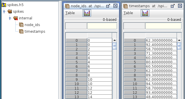
whrer N is the number of spikes. The group may contain an attribute “sorting” with values none, by_id, and by_time to indicate if and how the spikes are sorted (default none). There is also an optional attribute “units” for the timestamps, but defaults to milliseconds.
Reading#
You can use the SpikeTrains class to load
a sonata spikes files (or csv or nwb) into memory:
from bmtk.utils.reports.spike_trains import SpikeTrains

pop_name = ...
spikes = SpikeTrains.load('output/spikes.h5', population='pop_name')
assert(spikes.populations = [pop_name])
print(spikes.n_spikes())
print(spikes.node_ids())
If you know what node you want, use the get_times()
method to return an array of all spikes for a single node
node0_times = spikes.get_times(node_id=0)
print(node0_times)
Otherwise, you can use the to_dataframe()
or spikes() method to get a list of
all node_ids plus timestamps
for ts, pop, node_id in spikes():
   assert(pop == pop_name)
   ...
print(spikes.to_dataframe())
Plotting#
Analysis#
Creating Spike Trains#
Commonly it’s necessary to generate spike-trains to use as inputs for a simulation. One option is to use FilterNet to
generate inputs from external stimuli. You can also use the output of one simulation as the input to the next. But if
you need to generate your own spike files in SONATA format, BMTK provides two ways to do so. One
is to use the SpikeTrains class
add_spikes() or
add_spike() method:
from bmtk.utils.reports.spike_trains import SpikeTrains

spikes = SpikeTrains(population='my_inputs')
spikes.add_spikes(node_ids=0, timestamps=[1.0, 2.0, 3.0, ...])
spikes.add_spike(node_id=[1, 1, 2, 3],
                 timestamps=[0.5, 0.9, 1.0, 1.0])
Another is o use the PoissonSpikeGenerator class
from bmtk.utils.reports.spike_trains import PoissonSpikeGenerator

psg = PoissonSpikeGenerator(population='thalamus')
times = np.linspace(0.0, 3.0, 100000)
frs = 10*np.sin(times) + 5.0
psg.add(node_ids=range(10), firing_rate=frs, times=times)
psg.add(node_ids=range(10, 20), firing_rate=15.0, times=(0.0, 3.0))
psg.to_sonata('./inputs/thamlamus_inputs.h5')
Cell Variable Report#
Used to record the traces of intracellular and membrane variables throughout the simulation, like membrane potential V. In the HDF5, cell reports are stored under /report/<population_name>/ with the most relevant datasets:
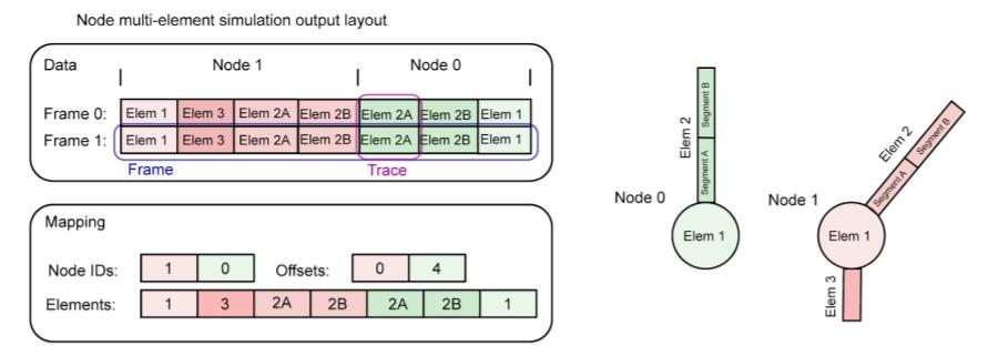
data (size T_times x N_segments): All the recorded values, with each row a different step in time and each column a different segment/cell
mapping/time (size 3 or T_times): For the exact times of each recording. If the simulation time steps are uniform, the dataset contains 3 values: start_time, stop_time, and time_step (all in ms). Otherwise, there will be of size T_times for each recording time since the start of the simulation.
mapping/node_ids: used to map each column to a specific cell
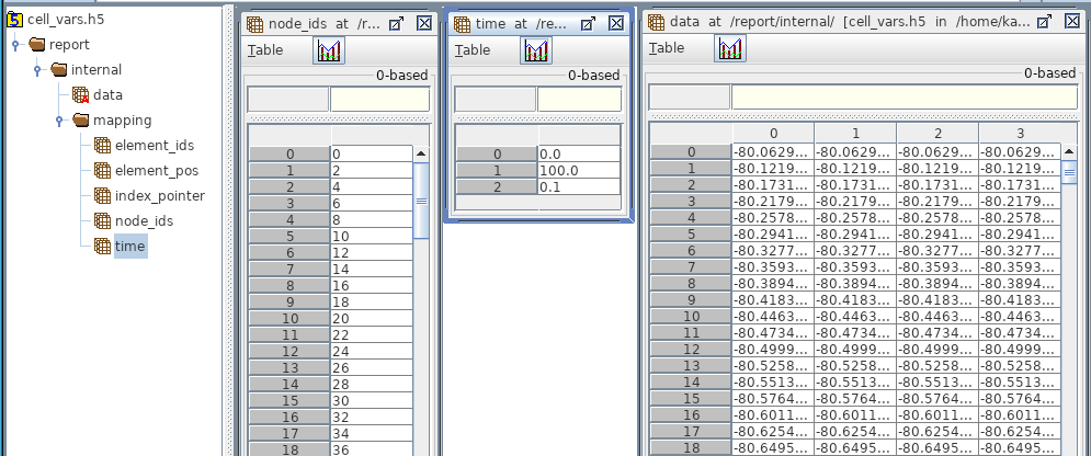
If the recording is done only on the soma or point-neurons, there will be one column in “data” for each node. If recording different sections from a multi-compartmental neuron then mapping/index_pointers can be used:
Reading Cell Variables#
The CompartmentReport class can be used to
read data from a cell report.
bmtk.utils.reports.compartment import CompartmentReport

pop_name = ...
report = CompartmentReport('output/membrane_vm.h5',
population=pop_name, mode='r')
print(report.variable())
print(report.tstart(), report.tstop(), report.dt())
print(report.element_ids(node_id=0))
print(report.element_pos(node_id=0))
print(report.data(node_id=0))
v
0.0, 3.0, 0.01
[0, 1, 2, 2, ...]
[0.5, 0.5, 0.5, 05, ...]
[[-50.010, -50.911, -50.995, -51.000, ...]
[-49.933, -49.330, -50.011, -50.667, ...]
...]