Adaptive and coordinated behavior requires that an animal be able to make predictions about the near and even far future. This intuition that some neural computations should be ‘predictive’ in their character has a long history, starting with ideas about how the receptive field structure of retinal ganglion cells relate to the statistics of natural visual scenes. Ideas about predictive computation have been most influential in thinking about the function of the neocortex. Here, the relatively stereotyped local circuitry of the neocortex has long led to speculation that each local circuit might be carrying out a somewhat similar, fundamental computation on its specific inputs. In addition, the organization of sensory-motor pathways into hierarchies (e.g., V1 V2 V4 IT in the ventral visual stream) with stereotyped feedforward and feedback connections has motivated ideas about hierarchical predictive codes, where higher levels of the hierarchy send predictions down to the lower level that then compares its inputs against the predictions and only send the surprises up the hierarchy (such as in the work of Mumford, Rao & Ballard, and Friston). Despite the wide influence of ideas about predictive coding, there is relatively little experimental evidence that such computations occur in multiple cortical areas, perhaps serving as a ‘canonical computation’ of the neocortical microcircuit. Our experimental design is based on a Sequence Learning Experiment, in which head-fixed mice passively view sequences of three different natural movie clips (labeled ‘A’, ‘B’, ‘C’), each having a duration of 2 seconds (Figure 1). We begin with one recording session (day #0), where the movie clips are presented in random order along with a 2 second grey screen (labeled ‘X’). Each stimulus occurs a total of 525 times, allowing a thorough characterization of neural responses before any sequence learning has occurred. Next, there are 3 recording sessions where the three movie clips are presented in a repeating temporal sequence, ABCABC…, for 500 times, in order to train the mouse’s brain. This training allows the mouse to potentially use the identity of the current movie clip predict the next movie clip. In addition, each sequence training session includes a period of random-order presentation, in order to assess changes in neural tuning during sequence learning. Finally, our last session (day #4) had stimuli presented in random order, allowing us to test more thoroughly how responses changed due to sequence learning.
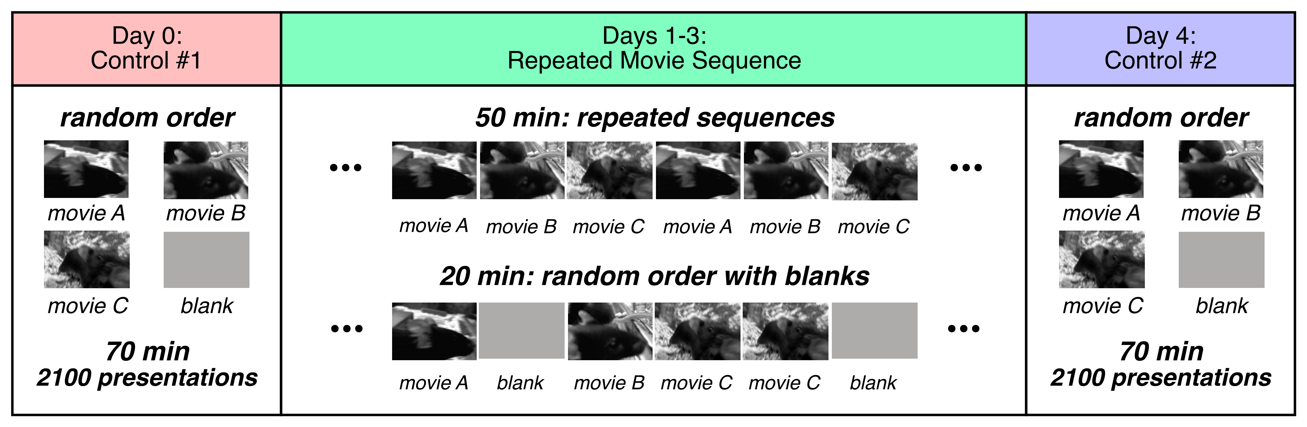
What makes the predictive coding hypothesis so powerful and interesting is the idea that these computations might be repeated in many different cortical microcircuits. Therefore, our design uses 2-photon microscopy with eight simultaneously recorded fields-of-view. The fields-of-view will include both layer 2/3 and layer 4 as well as from multiple cortical areas: V1 (VISp), LM (VISl), AM (VISam), and PM (VISpm).
In the ascending sensory pathway, signals enter layer 4 and then pass on to layer 2/3, before leaving for other cortical areas. Thus, layers 4 and 2/3 represent two different image processing steps with different tuning properties. For instance, in the primary visual cortex, neurons in layer 4 primarily have simple-cell receptive fields, while those in layer 2/3 primarily have complex-cell receptive fields. By recording simultaneously in both layers, we can compare the predictive computations present in these two stages of sensory processing in the local microcircuit.
The mouse visual system has roughly 10 visual areas organized into three hierarchical levels. Cortical area LM is thought to be most analogous to area V2 in the cat and primate, where the ventral stream is associated with processing ‘what’ an image is. Cortical area PM is an extra-striate area that may be related to the dorsal stream in cats and primates. Finally, cortical area AM is thought to be hierarchically higher than area PM. Together, these recordings from extra-striate visual areas allows us to compare the predictive computations present in different stages of the cortical hierarchy.
To these ends, the experiment used the Cux2-CreERTS2:Camk2a-tTa; Ai93(TITL-GCaMP6f) mouse line, which has expression in excitatory neurons of both layer 4 and 2/3.
Environment Setup
⚠️Note: If running on a new environment, run this cell once and then restart the kernel⚠️
import warnings
warnings.filterwarnings('ignore')

try:
    from databook_utils.dandi_utils import dandi_download_open
except:
    !git clone https://github.com/AllenInstitute/openscope_databook.git
    %cd openscope_databook
    %pip install -e .
    %cd docs/projects
import os
import matplotlib as mpl
import matplotlib.pyplot as plt
import numpy as np
import pandas as pd
from mpl_interactions import hyperslicer
from scipy import interpolate
from scipy.stats import ttest_ind
%matplotlib inlineThe Experiment
Here is an overview of the experimental sessions.
| Day | Stimulus | Cre Line | Depth | Visual Areas | Mice |
|---|---|---|---|---|---|
| 0 | random order | Cux2 | layer 2/3, 4 | VISp, VISl, VISam, VISpm | 13 |
| 1 | repeated sequence | Cux2 | layer 2/3, 4 | VISp, VISl, VISam, VISpm | 13 |
| 2 | repeated sequence | Cux2 | layer 2/3, 4 | VISp, VISl, VISam, VISpm | 13 |
| 3 | repeated sequence | Cux2 | layer 2/3, 4 | VISp, VISl, VISam, VISpm | 13 |
| 4 | random order | Cux2 | layer 2/3, 4 | VISp, VISl, VISam, VISpm | 13 |
For each mouse, we wanted to be able to compare the same neurons across different days. This meant that the field-of-view needed to be the same, which is technically challenging. The comparison between day #0 and day #4 was very important, but it was less important to record every day during the temporal sequence training. At the same time, it was important for all mice to receive a similar training profile. Even if a recording session did not match the initial field-of-view successfully, the animal still experienced the same passive visual exposure. Therefore, some animals did not have matching fields-of-view across all recording sessions.
In addition, it is important to be able to test what influence running has on observed predictive computations. This requires that an animal spent sufficient fractions of its session both running and not-running, in order to compare those two conditions. To this end, some sessions were repeated when the animal failed to run sufficiently. Priority was given to having sufficient running on the day #4 session. Thus, this session was repeated in a number of animals.
Overall, each of the 13 animals included in the DANDI Archive had a unique profile of recording sessions. For this release of the Sequential Learning project, Openscope has pre-released its session files on the DANDI Archive. The following table gives a summary of all the files from the 13 mice in this dataset. 8 files are produced from each experimental session, one for each imaging plane, and up to 6 sessions are conducted with each mouse. This table was generated from Getting Experimental Metadata from DANDI.
session_files = pd.read_csv("../../data/seqlearn_sessions.csv")
session_files# Function to convert string representation of a set to an actual set
def parse_set_string(set_string):
# Remove curly braces, split by commas, strip spaces and single quotes
return set(item.strip("'") for item in set_string.strip("{}").split(", "))
subjects = session_files.groupby('sub_name').agg(
n_sessions=('session_id', 'nunique'), # Count unique session IDs
stim_types=('stim_types', lambda x: set().union(*x.apply(parse_set_string))), # Union of all sets of stim_types
genotype=('sub_genotype', 'unique')
).reset_index()
subjectsn_sessions = len(session_files["session_id"].value_counts())
subjects_info = session_files.groupby(["specimen_name", "sub_sex"]).size().reset_index().to_dict()
m_count = len([sex for sex in subjects_info["sub_sex"].values() if sex == "M"])
f_count = len([sex for sex in subjects_info["sub_sex"].values() if sex == "F"])
print("Dandiset Overview:")
print(len(session_files), "files")
print(len(subjects_info["specimen_name"]), "subjects", m_count, "males", f_count,"females")Dandiset Overview:
1197 files
13 subjects 7 males 6 females
Downloading Ophys File
The files can be downloaded from the DANDI Archive. For a more detailed explanation of downloading and opening these files, see Downloading an NWB file. Here, we take one file for each of the stimulus regimes used in this project; the sequentially repeated stimulus and the randomly ordered stimulus.
dandiset_id = "000617"
sequence_dandi_filepath = "sub-688425/sub-688425_ses-1306855381-acq-1307046775_ophys.nwb"
random_dandi_filepath = "sub-688425/sub-688425_ses-1307534620-acq-1307650789_ophys.nwb"
download_loc = "."
# This can sometimes take a while depending on the size of the file
seq_io = dandi_download_open(dandiset_id, sequence_dandi_filepath, download_loc)
seq_nwb = seq_io.read()
# This can sometimes take a while depending on the size of the file
rand_io = dandi_download_open(dandiset_id, random_dandi_filepath, download_loc)
rand_nwb = rand_io.read()A newer version (0.67.1) of dandi/dandi-cli is available. You are using 0.61.2
File already exists
Opening file
File already exists
Opening file
# view the contents of the nwb interactively
seq_nwbImaging Data
Our Ophys files include lab metadata and imaging_planes objects which entail the information about the location being imaged, shown below. These files were chosen such that they are from the same mouse and were imaged at approximately the same depth.
print("Subject ID",seq_nwb.subject.subject_id)
print('Imaging Depth', seq_nwb.lab_meta_data['metadata'].imaging_depth)
print('Location', seq_nwb.imaging_planes['imaging_plane_1'].location)
Subject ID 688425
Imaging Depth 175
Location VISp
print("Subject ID",rand_nwb.subject.subject_id)
print('Imaging Depth', rand_nwb.lab_meta_data['metadata'].imaging_depth)
print('Location', rand_nwb.imaging_planes['imaging_plane_1'].location)
Subject ID 688425
Imaging Depth 180
Location VISp
Stimulus Templates
The files for the Sequential Learning project contain the movies used as visual stimulus, referred to as stim templates. The project contain three main stimulus movies with regular forward playback. Below, screenshots from each of the movies are displayed, and one of the movies can be played embedded within this notebook. The key used can be changed to view different stim templates.
seq_nwb.stimulus_template.keys()dict_keys(['gray', 'movie_clip_A', 'movie_clip_B', 'movie_clip_C'])n_cols = 2
n_rows = 2
fig, axes = plt.subplots(n_rows, n_cols, figsize=(n_cols*2, n_rows*2))
if len(axes.shape) == 1:
axes = axes.reshape((1, axes.shape[0]))
for i, template_name in enumerate(seq_nwb.stimulus_template.keys()):
template_img = seq_nwb.stimulus_template[template_name].data[:,:,0]
template_img = np.rot90(template_img, k=3)
ax_row = int(i / n_cols)
ax_col = i % n_cols
axes[ax_row][ax_col].imshow(template_img, cmap="gray")
axes[ax_row][ax_col].set_title(template_name, fontsize=8)
for ax in axes.flat:
ax.xaxis.set_ticks([])
ax.yaxis.set_ticks([])
fig.tight_layout()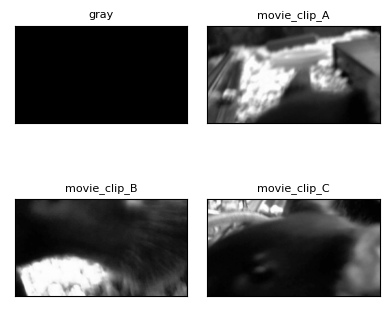
%matplotlib ipympl
plt.tick_params(left=False, bottom=False, labelleft=False, labelbottom=False)

# change this key to view other stim template movies
template_key = "movie_clip_B"
template = seq_nwb.stimulus_template[template_key].data
template = np.transpose(template)
view = hyperslicer(template, play_buttons=True, cmap="gray")Selecting Stimulus Times
In order to analyze the data, the precise timing of the stimulus is required. This information is stored in a set of tables, one for each stimulus video. These are used to select trial times of interest.
Overall, information about the stimulus is organized as follows:
There are separate folders containing timing information for each of the 4 different stimuli: ‘gray_presentations’ ‘movie_clip_A_presentations’ ‘movie_clip_B_presentations’ ‘movie_clip_C_presentations’
Within each folder, there are the following lists: ‘id’: a unique integer identifying a presentation frame, runs from 0 to ~63,000 ‘frame’: an integer describing which frame within the movie clip is presented this runs from 0 to 119, repeating periodically, once per movie clip ‘start_time’: time at which each frame starts this number has stretches that increment by 1/60 Hz ~ 0.01667 sec separated by larger jumps, where other stimuli are presented ‘stop_time’: time at which each frame stops; similar format to ‘start_time’ ‘stim_block’: contains an integer describing the presentation order of the current movie clip this number runs from 0 to 2099; it has constant stretches interspersed with jumps
In order to find the set of times at which a given movie clip is presented, look for ‘start_times’ subject to the condition that ‘frame’ = 0. For other analysis,
seq_stim_selectandrand_stim_selectcan below, can be modified to select different stimulus times.
print(seq_nwb.intervals.keys())
print(rand_nwb.intervals.keys())
dict_keys(['gray_presentations', 'movie_clip_A_presentations', 'movie_clip_B_presentations', 'movie_clip_C_presentations'])
dict_keys(['gray_presentations', 'movie_clip_A_presentations', 'movie_clip_B_presentations', 'movie_clip_C_presentations'])
seq_stim_table = seq_nwb.intervals["movie_clip_B_presentations"]
seq_stim_table[:10]print("Frame nums:", set(seq_stim_table.frame))
seq_stim_select = lambda row: row.frame.item() == 0.0
seq_stim_times = [float(seq_stim_table[i].start_time) for i in range(len(seq_stim_table)) if seq_stim_select(seq_stim_table[i])]
print("Selected stim times:", len(seq_stim_times))Frame nums: {0.0, 1.0, 2.0, 3.0, 4.0, 5.0, 6.0, 7.0, 8.0, 9.0, 10.0, 11.0, 12.0, 13.0, 14.0, 15.0, 16.0, 17.0, 18.0, 19.0, 20.0, 21.0, 22.0, 23.0, 24.0, 25.0, 26.0, 27.0, 28.0, 29.0, 30.0, 31.0, 32.0, 33.0, 34.0, 35.0, 36.0, 37.0, 38.0, 39.0, 40.0, 41.0, 42.0, 43.0, 44.0, 45.0, 46.0, 47.0, 48.0, 49.0, 50.0, 51.0, 52.0, 53.0, 54.0, 55.0, 56.0, 57.0, 58.0, 59.0, 60.0, 61.0, 62.0, 63.0, 64.0, 65.0, 66.0, 67.0, 68.0, 69.0, 70.0, 71.0, 72.0, 73.0, 74.0, 75.0, 76.0, 77.0, 78.0, 79.0, 80.0, 81.0, 82.0, 83.0, 84.0, 85.0, 86.0, 87.0, 88.0, 89.0, 90.0, 91.0, 92.0, 93.0, 94.0, 95.0, 96.0, 97.0, 98.0, 99.0, 100.0, 101.0, 102.0, 103.0, 104.0, 105.0, 106.0, 107.0, 108.0, 109.0, 110.0, 111.0, 112.0, 113.0, 114.0, 115.0, 116.0, 117.0, 118.0, 119.0}
Selected stim times: 525
rand_stim_table = rand_nwb.intervals["movie_clip_B_presentations"]
rand_stim_table[:10]print("Frame nums:", set(rand_stim_table.frame))
rand_stim_select = lambda row: row.frame.item() == 0.0
rand_stim_times = [float(rand_stim_table[i].start_time) for i in range(len(rand_stim_table)) if rand_stim_select(rand_stim_table[i])]
print("Selected stim times:", len(rand_stim_times))Frame nums: {0.0, 1.0, 2.0, 3.0, 4.0, 5.0, 6.0, 7.0, 8.0, 9.0, 10.0, 11.0, 12.0, 13.0, 14.0, 15.0, 16.0, 17.0, 18.0, 19.0, 20.0, 21.0, 22.0, 23.0, 24.0, 25.0, 26.0, 27.0, 28.0, 29.0, 30.0, 31.0, 32.0, 33.0, 34.0, 35.0, 36.0, 37.0, 38.0, 39.0, 40.0, 41.0, 42.0, 43.0, 44.0, 45.0, 46.0, 47.0, 48.0, 49.0, 50.0, 51.0, 52.0, 53.0, 54.0, 55.0, 56.0, 57.0, 58.0, 59.0, 60.0, 61.0, 62.0, 63.0, 64.0, 65.0, 66.0, 67.0, 68.0, 69.0, 70.0, 71.0, 72.0, 73.0, 74.0, 75.0, 76.0, 77.0, 78.0, 79.0, 80.0, 81.0, 82.0, 83.0, 84.0, 85.0, 86.0, 87.0, 88.0, 89.0, 90.0, 91.0, 92.0, 93.0, 94.0, 95.0, 96.0, 97.0, 98.0, 99.0, 100.0, 101.0, 102.0, 103.0, 104.0, 105.0, 106.0, 107.0, 108.0, 109.0, 110.0, 111.0, 112.0, 113.0, 114.0, 115.0, 116.0, 117.0, 118.0, 119.0}
Selected stim times: 650
Extracting ROI Fluorescence
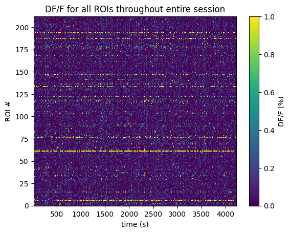
Below the 2-Photon Fluorescence data is extracted. Firstly, the imaging FOV for one session is shown with the session’s average projection, as well as the output of our cell segmentation algorithm, which identifies the cells (called regions-of-interest, or ROIs) from which the fluorescence traces were recorded. The raw fluorescence is normalized into DF/F % in order to eliminate sources of noise and day-to-day variability. The seq_dff_trace and rand_dff_trace arrays are 2D arrays pulled from the files which contain these recordings throughout the session for each ROI. They should have a shape (n_measurments x n_rois). They come with their respective arrays, seq_dff_timestamps and rand_dff_timestamps, that record the timestamp at which each measurement was taken.
%matplotlib inline
fig, axes = plt.subplots(1,2, figsize=(10,30))
axes[0].imshow(rand_nwb.processing['ophys']['images']['max_projection'])
axes[1].imshow(rand_nwb.processing['ophys']['images']['segmentation_mask_image'])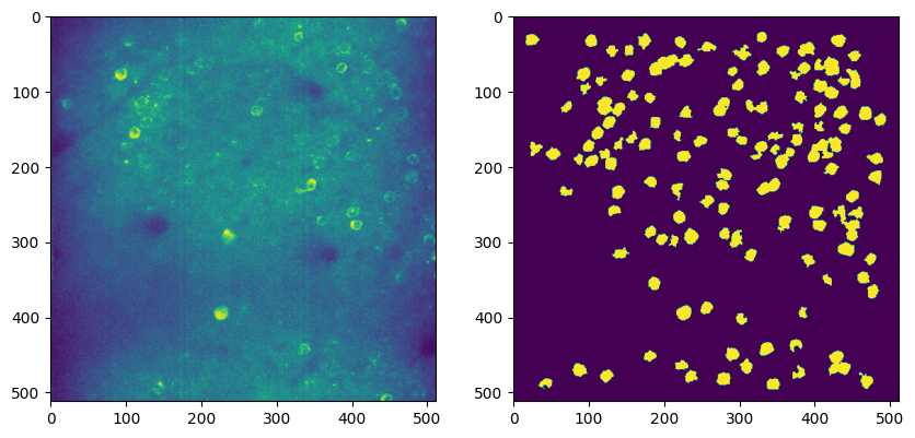
seq_dff = seq_nwb.processing["ophys"]["dff"]
seq_dff_trace = np.array(seq_dff.roi_response_series["traces"].data)
seq_dff_timestamps = np.array(seq_dff.roi_response_series["traces"].timestamps)

print(seq_dff_trace.shape)
print(seq_dff_timestamps.shape)

seq_avg_dff_trace = np.average(seq_dff_trace, axis=1)
(39978, 212)
(39978,)
rand_dff = rand_nwb.processing["ophys"]["dff"]
rand_dff_trace = np.array(rand_dff.roi_response_series["traces"].data)
rand_dff_timestamps = np.array(rand_dff.roi_response_series["traces"].timestamps)

print(rand_dff_trace.shape)
print(rand_dff_timestamps.shape)

rand_avg_dff_trace = np.average(rand_dff_trace, axis=1)
(39977, 145)
(39977,)
%matplotlib inline
n_rois = seq_dff_trace.shape[1]
plt.imshow(seq_dff_trace.transpose(), extent=[seq_dff_timestamps[0], seq_dff_timestamps[-1], 0, n_rois], aspect='auto', vmin=0, vmax=1, interpolation='None')
# plt.yticks(np.arange(n_rois)+0.5, np.arange(n_rois))
plt.ylabel("ROI #")
plt.xlabel("time (s)")
plt.title("DF/F for all ROIs throughout entire session")
cbar = plt.colorbar()
cbar.set_label('DF/F (%)')
Extracting Running
The recording of the mouse’s running on the wheel is also recorded as an array with accompanying timestamps, shown below.
seq_running = seq_nwb.processing["running"]["speed"]
seq_running_trace = np.array(seq_running.data)
seq_running_timestamps = np.array(seq_running.timestamps)

print(seq_running_trace.shape)
print(seq_running_timestamps.shape)
(252000,)
(252000,)
rand_running = rand_nwb.processing["running"]["speed"]
rand_running_trace = np.array(rand_running.data)
rand_running_timestamps = np.array(rand_running.timestamps)

print(rand_running_trace.shape)
print(rand_running_timestamps.shape)
(252000,)
(252000,)
plt.plot(seq_running_timestamps, seq_running_trace)
plt.xlabel("Time (s)")
plt.ylabel("Speed (cm/s)")
plt.title("Mouse running throughout session")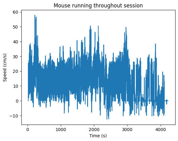
Session Timeline
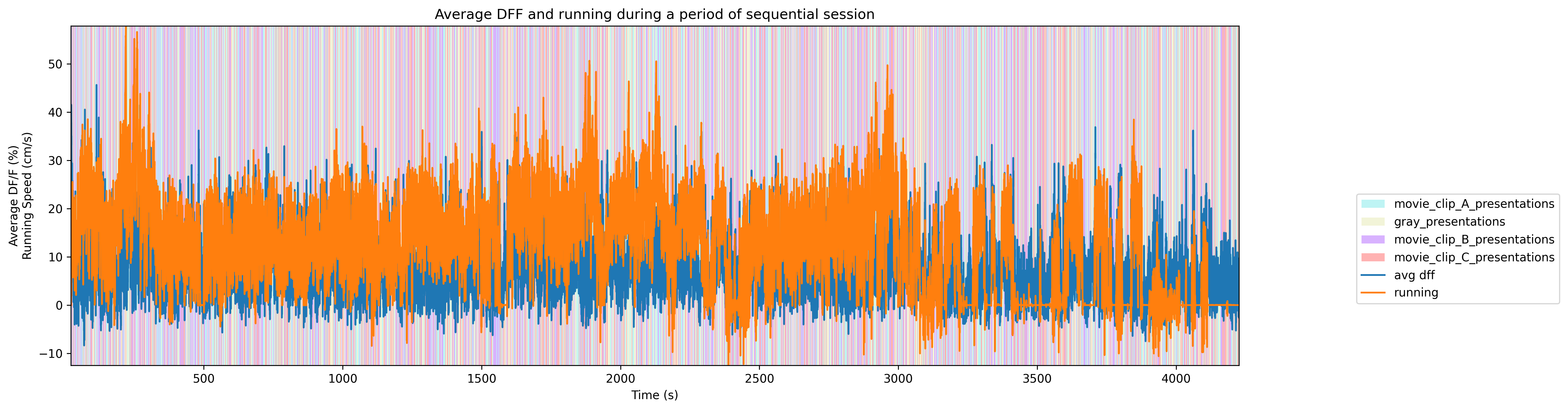
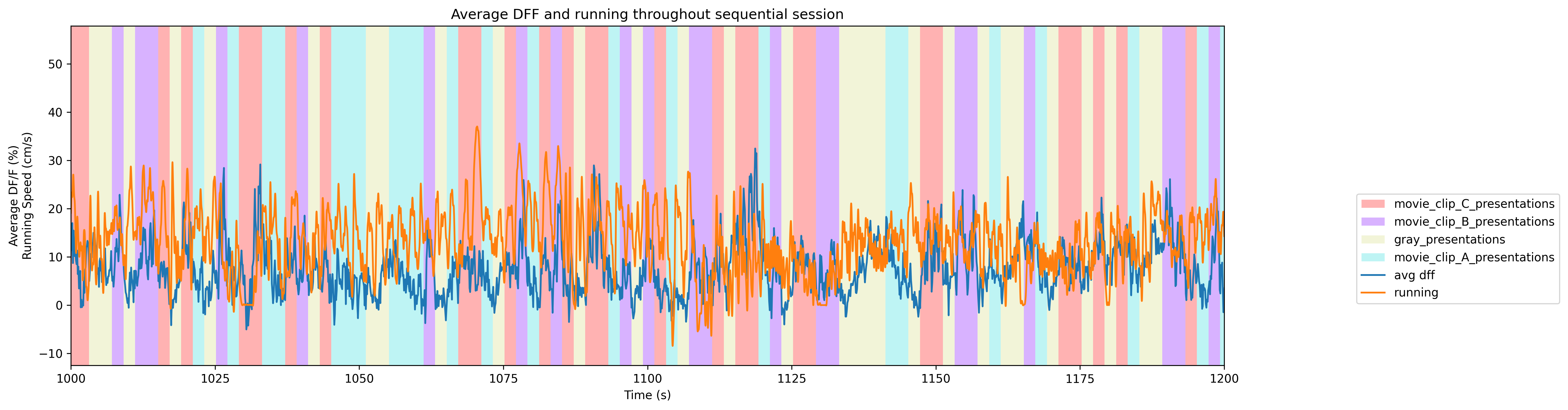
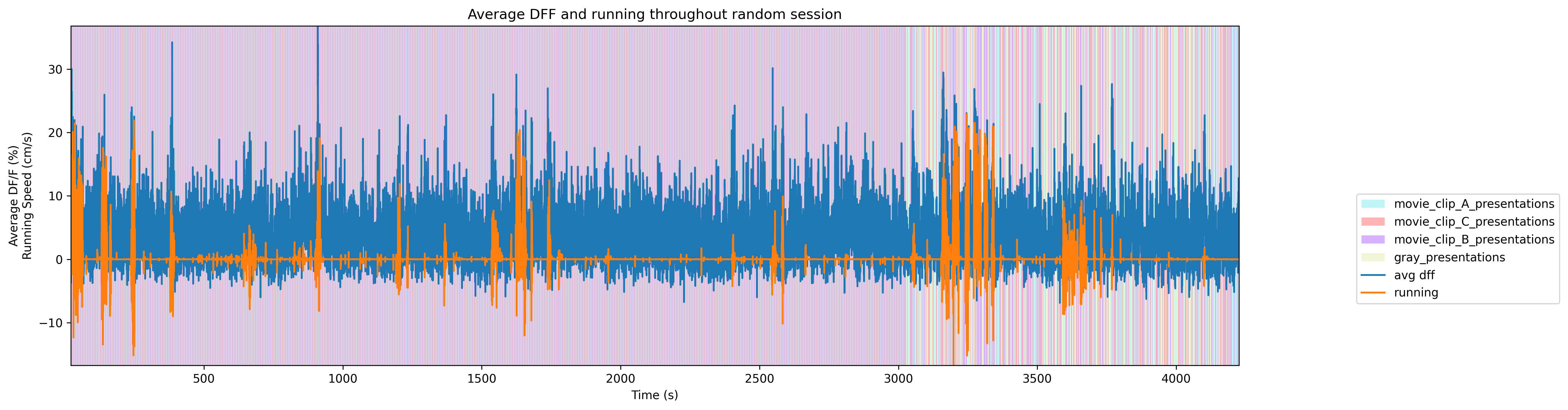
To get a good idea of the order and the way stimulus is shown throughout the session, the code below generates a timeline of the various ‘epochs’ of stimulus. It can be seen that the sessions either have fully randomized order of the three stim movies and grey, or a repeated sequence of the three movies. Note that due to the way the plot draws and mixes thin bands of color, the epochs in the sequential plot might seem like large blocks, when in fact they repeat quickly. A zoomed-in plot is shown for a clearer view.
# extract epoch times from stim table where stimulus rows have a different 'block' than following row
# returns list of epochs, where an epoch is of the form (stimulus name, stimulus block, start time, stop time)
def extract_epochs_from_table(stim_name, stim_table, epochs):

    # specify a current epoch stop and start time
    epoch_start = stim_table.start_time[0]
    epoch_stop = stim_table.stop_time[0]

    # for each row, try to extend current epoch stop_time
    for i in range(len(stim_table)):
        this_block = stim_table.stimulus_block[i]
        # if end of table, end the current epoch
        if i+1 >= len(stim_table):
            epochs.append((stim_name, this_block, epoch_start, epoch_stop))
            break

        next_block = stim_table.stimulus_block[i+1]
        # if next row is the same stim block, push back epoch_stop time
        if next_block == this_block:
            epoch_stop = stim_table.stop_time[i+1]
        # otherwise, end the current epoch, start new epoch
        else:
            epochs.append((stim_name, this_block, epoch_start, epoch_stop))
            epoch_start = stim_table.start_time[i+1]
            epoch_stop = stim_table.stop_time[i+1]

    return epochs
def extract_all_epochs(nwb):
# extract epochs from all valid stimulus tables
epochs = []
for stim_name in nwb.intervals.keys():
stim_table = nwb.intervals[stim_name]
try:
epochs = extract_epochs_from_table(stim_name, stim_table, epochs)
except:
continue
return epochs%matplotlib inline
### make plot of chosen trace over time with colored epoch sections
def plot_trace_over_epochs(trace_arrs, timestamps_arrs, epochs, time_start=None, time_end=None, title=None, trace_labels=None, yaxlabels=None, xlabel=None):
assert len(trace_arrs) == len(timestamps_arrs), "there must be an equal number of traces and timestamps arrays"
if trace_labels is not None:
assert len(trace_arrs) == len(trace_labels), "there must be an equal number of traces and trace labels arrays"
if yaxlabels is not None:
assert len(trace_arrs) == len(yaxlabels), "there must be an equal number of traces and y-axis labels arrays"
fig, ax = plt.subplots(figsize=(15,5), dpi=300)
if time_start is None:
time_start = np.min(np.concatenate(timestamps_arrs))
if time_end is None:
time_end = np.max(np.concatenate(timestamps_arrs))
# filter epochs which aren't at least partially in the time window
bounded_epochs = {epoch for epoch in epochs if epoch[2] < time_end and epoch[3] > time_start}
# assign unique color to each stimulus name
stim_names = list({epoch[0] for epoch in bounded_epochs})
colors = plt.cm.rainbow(np.linspace(0,1,len(stim_names)))
stim_color_map = {stim_names[i]:colors[i] for i in range(len(stim_names))}
key = {}
y_hi = np.max(np.concatenate(trace_arrs)) # change these to manually set height of the plot
y_lo = np.min(np.concatenate(trace_arrs))
# draw colored rectangles for each epoch
for epoch in bounded_epochs:
stim_name, stim_block, epoch_start, epoch_end = epoch
color = stim_color_map[stim_name]
rec = ax.add_patch(mpl.patches.Rectangle((epoch_start, y_lo), epoch_end-epoch_start, 100, alpha=0.3, facecolor=color, antialiased=False))
key[(stim_name)] = rec
ax.set_xlim(time_start, time_end)
ax.set_ylim(y_lo, y_hi)
if xlabel is not None:
ax.set_xlabel(xlabel)
if title is not None:
ax.set_title(title)
if yaxlabels is not None:
ax.set_ylabel("\n".join(yaxlabels))
for i in range(len(trace_arrs)):
# next_color = plt.rcParams["axes.prop_cycle"].by_key()["color"][i]
# this_ax = ax.twinx()
line = ax.plot(timestamps_arrs[i], trace_arrs[i])[0]
if trace_labels is not None:
key[(trace_labels[i])] = line
print(key)
fig.legend(key.values(), key.keys(), loc="lower right", bbox_to_anchor=(1.25, 0.25))
return axseq_epochs = extract_all_epochs(seq_nwb)
# epochs take the form (stimulus name, stimulus block, start time, stop time)
print("Num epochs:",len(seq_epochs))
seq_epochs.sort(key=lambda x: x[2])
for epoch in seq_epochs:
print(epoch)
# can set these manually to get a closer look at the timeline
time_start = min(seq_epochs, key=lambda epoch: epoch[1])[1]
time_end = max(seq_epochs, key=lambda epoch:epoch[2])[2]
# time_start = 3000
# time_end = 3100
# can set this to change what trace is displayed alongside epochs
display_trace = seq_avg_dff_trace * 100 # to yield percentage
# unit_idx = 30
# display_trace = dff_trace[:,unit_idx] * 100# adjust these to zoom in to a narrow slice of time
start, stop = None, None
ax = plot_trace_over_epochs([display_trace, seq_running_trace], [seq_dff_timestamps, seq_running_timestamps], seq_epochs, start, stop, "Average DFF and running during a period of sequential session", ['avg dff', 'running'], ["Average DF/F (%)","Running Speed (cm/s)"], "Time (s)")
plt.tight_layout()
plt.show(){'movie_clip_A_presentations': <matplotlib.patches.Rectangle object at 0x0000021BE9A662F0>, 'gray_presentations': <matplotlib.patches.Rectangle object at 0x0000021BE9A65D50>, 'movie_clip_B_presentations': <matplotlib.patches.Rectangle object at 0x0000021BE9A65F30>, 'movie_clip_C_presentations': <matplotlib.patches.Rectangle object at 0x0000021BE9A65990>, 'avg dff': <matplotlib.lines.Line2D object at 0x0000021BE9A665C0>, 'running': <matplotlib.lines.Line2D object at 0x0000021BE9A66860>}
# adjust these to zoom in to a narrow slice of time
start, stop = 1000, 1200
ax = plot_trace_over_epochs([display_trace, seq_running_trace], [seq_dff_timestamps, seq_running_timestamps], seq_epochs, start, stop, "Average DFF and running throughout sequential session", ['avg dff', 'running'], ["Average DF/F (%)","Running Speed (cm/s)"], "Time (s)")
plt.tight_layout()
plt.show()
{'movie_clip_C_presentations': <matplotlib.patches.Rectangle object at 0x0000021BEC00C5B0>, 'movie_clip_B_presentations': <matplotlib.patches.Rectangle object at 0x0000021BEBFC7A30>, 'gray_presentations': <matplotlib.patches.Rectangle object at 0x0000021BEC00C790>, 'movie_clip_A_presentations': <matplotlib.patches.Rectangle object at 0x0000021BEC00C970>, 'avg dff': <matplotlib.lines.Line2D object at 0x0000021BEC00CC40>, 'running': <matplotlib.lines.Line2D object at 0x0000021BEC00CEE0>}
rand_epochs = extract_all_epochs(rand_nwb)

# epochs take the form (stimulus name, stimulus block, start time, stop time)
print("Num epochs:",len(rand_epochs))
rand_epochs.sort(key=lambda x: x[2])
# for epoch in rand_epochs:
#     print(epoch)

# can set these manually to get a closer look at the timeline
time_start = min(rand_epochs, key=lambda epoch: epoch[1])[1]
time_end = max(rand_epochs, key=lambda epoch:epoch[2])[2]
# time_start = 3000
# time_end = 3100

# can set this to change what trace is displayed alongside epochs
display_trace = rand_avg_dff_trace * 100 # to yield percentage
# unit_idx = 30
# display_trace = dff_trace[:,unit_idx] * 100

# adjust these to zoom in to a narrow slice of time
start, stop = None, None
ax = plot_trace_over_epochs([display_trace, rand_running_trace], [rand_dff_timestamps, rand_running_timestamps], rand_epochs, start, stop, "Average DFF and running throughout random session", ['avg dff', 'running'], ["Average DF/F (%)","Running Speed (cm/s)"], "Time (s)")
plt.tight_layout()
plt.show()
Num epochs: 2100
{'movie_clip_A_presentations': <matplotlib.patches.Rectangle object at 0x0000021BE9908B80>, 'movie_clip_C_presentations': <matplotlib.patches.Rectangle object at 0x0000021BE9909120>, 'movie_clip_B_presentations': <matplotlib.patches.Rectangle object at 0x0000021BE99087C0>, 'gray_presentations': <matplotlib.patches.Rectangle object at 0x0000021BE9908F40>, 'avg dff': <matplotlib.lines.Line2D object at 0x0000021BE99093F0>, 'running': <matplotlib.lines.Line2D object at 0x0000021BE9909690>}
Generating Response Windows
With the selected trial times above, seq_stim_times and rand_stim_times, aligned responses to these trials throughout the session can be plotted. To align in time, the DF/F traces must first be interpolated. The code below calculates these ‘neuronwise response windows’.
window_start_time = -2
window_end_time = 3
interp_hz = 10
# generate regularly-space x values and interpolate along it
time_axis = np.arange(seq_dff_timestamps[0], seq_dff_timestamps[-1], step=(1/interp_hz))
interp_dff = []
# interpolate channel by channel to save RAM
for channel in range(seq_dff_trace.shape[1]):
f = interpolate.interp1d(seq_dff_timestamps, seq_dff_trace[:,channel], axis=0, kind="nearest", fill_value="extrapolate")
interp_dff.append(f(time_axis))
interp_dff = np.array(interp_dff)
print(interp_dff.shape)(212, 42046)
# validate window bounds
if window_start_time > 0:
    raise ValueError("start time must be non-positive number")
if window_end_time <= 0:
    raise ValueError("end time must be positive number")

# get event windows
windows = []
window_length = int((window_end_time-window_start_time) * interp_hz)

for stim_ts in seq_stim_times:
    # convert time to index
    start_idx = int( (stim_ts + window_start_time - seq_dff_timestamps[0]) * interp_hz )
    end_idx = start_idx + window_length

    # bounds checking
    if start_idx < 0 or end_idx > interp_dff.shape[1]:
        continue

    windows.append(interp_dff[:,start_idx:end_idx])

if len(windows) == 0:
    raise ValueError("There are no windows for these timestamps")

windows = np.array(windows) * 100 # x100 to convert values to dF/F percentage
neuronwise_windows = np.swapaxes(windows,0,1)

print(neuronwise_windows.shape)
(212, 525, 50)
Showing Response Windows
%matplotlib inline
def show_dff_response(ax, dff, window_start_time, window_end_time, aspect="auto", vmin=None, vmax=None, yticklabels=[], skipticks=1, xlabel="Time (s)", ylabel="ROI", cbar=True, cbar_label=None):
    if len(dff) == 0:
        print("Input data has length 0; Nothing to display")
        return

    img = ax.imshow(dff, aspect=aspect, extent=[window_start_time, window_end_time, 0, len(dff)], vmin=vmin, vmax=vmax)
    if cbar:
        ax.colorbar(img, shrink=0.5, label=cbar_label)

    ax.plot([0,0],[0, len(dff)], ":", color="white", linewidth=1.0)

    if len(yticklabels) != 0:
        ax.set_yticks(range(len(yticklabels)))
        ax.set_yticklabels(yticklabels, fontsize=8)

        n_ticks = len(yticklabels[::skipticks])
        ax.yaxis.set_major_locator(plt.MaxNLocator(n_ticks))

    ax.set_xlabel(xlabel)
    ax.set_ylabel(ylabel)
def show_many_responses(windows, rows, cols, window_idxs=None, title=None, subplot_title="", xlabel=None, ylabel=None, cbar_label=None, vmin=0, vmax=100):
if window_idxs is None:
window_idxs = range(len(windows))
windows = windows[window_idxs]
# handle case with no input data
if len(windows) == 0:
print("Input data has length 0; Nothing to display")
return
# handle cases when there aren't enough windows for number of rows
if len(windows) < rows*cols:
rows = (len(windows) // cols) + 1
fig, axes = plt.subplots(rows, cols, figsize=(2*cols+2, 2*rows+2), layout="constrained")
# handle case when there's only one row
if len(axes.shape) == 1:
axes = axes.reshape((1, axes.shape[0]))
for i in range(rows*cols):
ax_row = int(i // cols)
ax_col = i % cols
ax = axes[ax_row][ax_col]
if i > len(windows)-1:
ax.set_visible(False)
continue
window = windows[i]
show_dff_response(ax, window, window_start_time, window_end_time, xlabel=xlabel, ylabel=ylabel, cbar=False, vmin=vmin, vmax=vmax)
ax.set_title(f"{subplot_title} {window_idxs[i]}")
if ax_row != rows-1:
ax.get_xaxis().set_visible(False)
if ax_col != 0:
ax.get_yaxis().set_visible(False)
fig.suptitle(title)
norm = mpl.colors.Normalize(vmin=vmin, vmax=vmax)
colorbar = fig.colorbar(mpl.cm.ScalarMappable(norm=norm), ax=axes, shrink=1.5/rows, label=cbar_label)show_many_responses(neuronwise_windows,
6,
15,
title="Response of Some ROIs across trials",
subplot_title="ROI",
xlabel="time (s)",
ylabel="trial",
cbar_label="$\Delta$F/F (%)")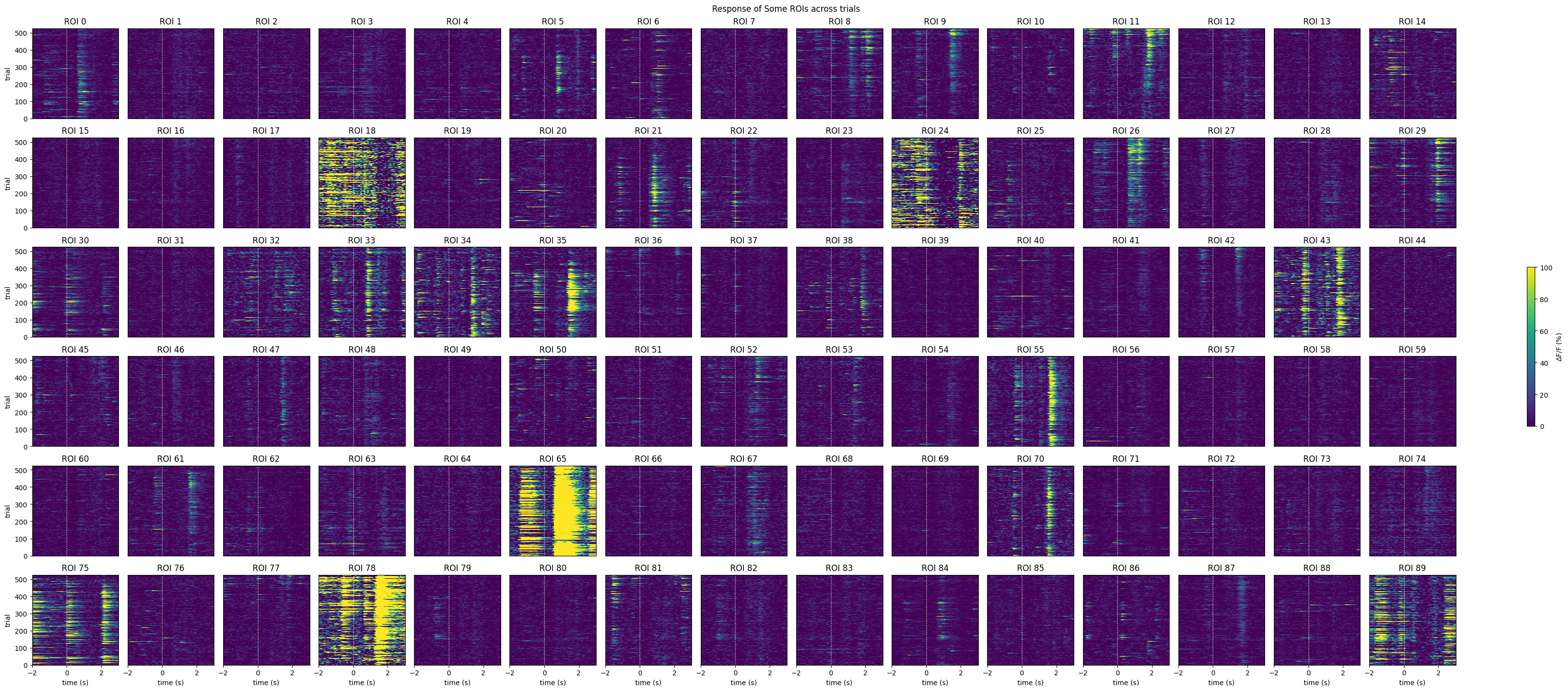
Selecting Cells
# get the index within the window that stimulus occurs (time 0)
stimulus_onset_idx = int(-window_start_time * interp_hz)
baseline = windows[:,:,0:stimulus_onset_idx]
evoked_responses = windows[:,:,stimulus_onset_idx:]

print(stimulus_onset_idx)
print(baseline.shape)
print(evoked_responses.shape)
20
(525, 212, 20)
(525, 212, 30)
mean_trial_responses = np.mean(evoked_responses, axis=2)
mean_trial_baselines = np.mean(baseline, axis=2)

n = mean_trial_responses.shape[0]
t,p = ttest_ind(mean_trial_responses, mean_trial_baselines)
IC3_selected_rois = np.where(p < 0.05 / n)[0]
print(f"Selected ROIs {IC3_selected_rois}")
Selected ROIs [ 1 5 8 11 12 14 18 21 23 24 25 26 29 35 47 55 61 62
65 67 68 70 78 87 89 91 92 93 95 105 108 115 119 122 123 125
127 129 130 132 134 137 140 142 144 148 149 155 156 164 168 171 174 180
182 183 186 194 197 200 205 207 209]
show_many_responses(neuronwise_windows[IC3_selected_rois],
                    6,
                    15,
                    title="Response of Some ROIs across trials",
                    subplot_title="ROI",
                    xlabel="time (s)",
                    ylabel="trial",
                    cbar_label="$\Delta$F/F (%)")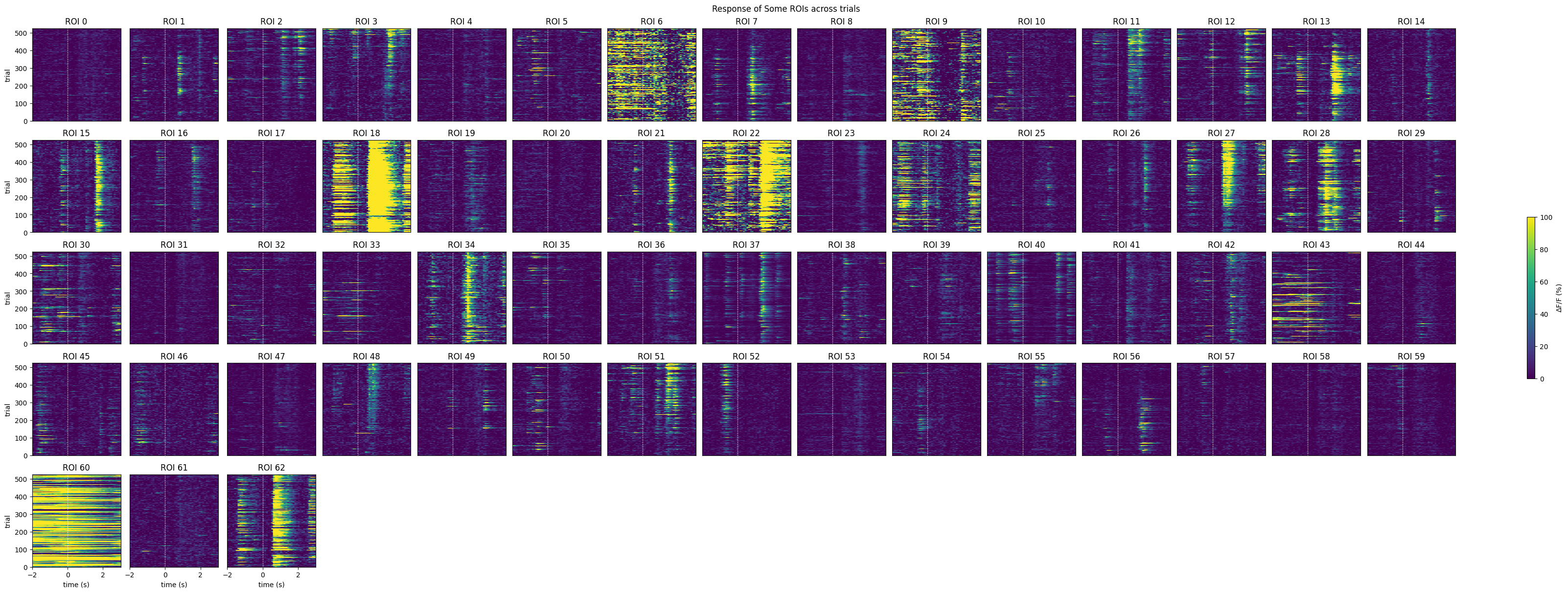
Viewing Raw Movie
Although not shown in the metadata table shown above, each one of our session files comes with a copy on DANDI that also includes the actual movies from the brain. This is downloaded and displayed below.
dandi_movie_filepath = "sub-688425/sub-688425_ses-1306855381-acq-1307046775-raw-movies_ophys.nwb"# This can sometimes take a while depending on the size of the file
io = dandi_download_open(dandiset_id, dandi_movie_filepath, download_loc)
nwb = io.read()File already exists
Opening file
# start_time = flr_timestamps[0]
start_time = 540
# end_time = flr_timestamps[-1]
end_time = 600
start_idx, end_idx = np.searchsorted(seq_dff_timestamps, [start_time, end_time])
print(start_idx)
print(end_idx)4928
5499
raw_movie = nwb.acquisition["raw_suite2p_motion_corrected"].data
flr_timestamps = np.array(seq_dff.roi_response_series["traces"].timestamps)

print(raw_movie.shape)
print(flr_timestamps.shape)
(39978, 512, 512)
(39978,)
%matplotlib ipympl
plt.tick_params(left=False, bottom=False, labelleft=False, labelbottom=False)
view = hyperslicer(raw_movie[start_idx:end_idx], play_buttons=True)