Project Overview
The OpenScope Community Predictive Processing project investigates how the brain anticipates and responds to violations of sensory expectations — a core idea in predictive processing theory. The central hypothesis is that the brain continuously builds internal models of the sensory world, and that neural activity is shaped not just by what the eyes see, but by the difference between what was predicted and what actually occurred.
This project is fully described in:
Neural mechanisms of predictive processing: a collaborative community experiment through the OpenScope program arXiv:2504.09614
Specific Aims
The Specific Aim of this proposal is to elucidate the potential relationship between four most commonly studied mismatch stimuli and their associated error signals, as well as different neuronal implementations of predictive processing.
Hypothesis-Driven Framework
We hypothesize that…
H0: Mechanisms of predictive processing fundamentally differ depending on predictive set and prediction error types, and recruit different neuronal mechanisms.
Alternatively, we hypothesize that…
H1: A unified predictive processing mechanism drives all mismatch processing in the mammalian cortex.
To determine which of these two alternative hypotheses is correct, we propose to experimentally examine three major types of mismatch stimuli that have dominated the literature: temporal, motor, and omission. Further, we will examine two types of prediction sets: spatiotemporal (passive) and sensorimotor (active). Importantly, in all experiments, the region recorded (V1) will include spatially intermixed neurons selective for features of both the expected stimulus and the mismatch stimuli. For example, orientation and direction tuning are spatially mixed in V1, and the standard oddball paradigms Zhou et al. (2020); Hamm et al. (2021); Pak et al. (2021); Homann et al. (2022) and sensorimotor mismatch paradigms Jordan & Keller (2020) involve predicted stimuli and mismatch stimuli that differ in orientation or direction.
Significance and Innovation
We will collect the first comprehensive set of neuronal data enabling direct comparison across different mismatch error signals. Additionally, our methodology will be designed to integrate two-photon imaging and electrophysiological recordings, leveraging the strengths of both techniques. Resolving these alternative hypotheses will mark major progress for the field, unifying conflicting findings and clarifying how differences in experimental design shape interpretations of predictive processing.
Additionally, the resulting dataset will be a pivotal resource for validating mechanistic computational models across multiple mismatch types, advancing our understanding of predictive processing in the brain.
Proposed Experiment
1. Stimulus Set Design
Our stimulus set will be designed to contain a few validated mismatch stimuli. Particular attention will be given to the experimental design to allow fitting models of:
Synaptic adaptation
Positive and negative errors
Short-term memory that could emerge through local recurrence
E/I balance
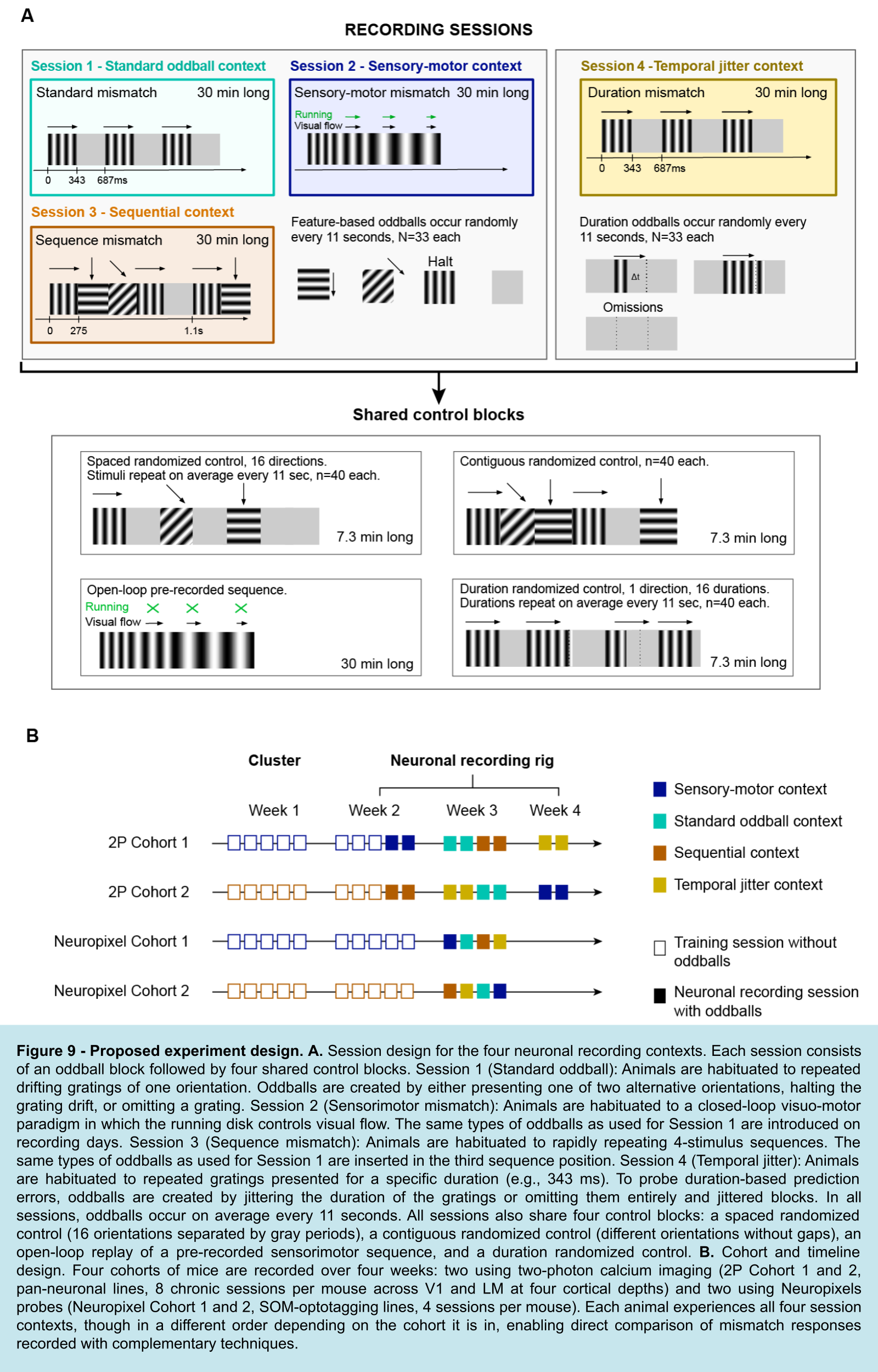
Since we aim to bridge various visual stimuli designs piloted, analyzed, and deployed over the last decades, we will use sequences of drifting gratings. We will present five types of oddballs: a drifting grating halt, two alternative drifting orientations, an omission, and temporal jittered oddballs. All oddballs will be introduced in four different session contexts: standard mismatch, sensory-motor mismatch, sequential mismatch, and temporal jitter mismatch. These contexts will be separated based on the session and habituation design. Individual animals will experience all 4 contexts in different orders. Two cohorts of separate animals will be recorded with Neuropixels probes and multi-area two-photon imaging.
Session 1 – Standard Mismatch: Animals will be habituated to a series of drifting gratings of the same orientation. Various mismatch stimuli will be introduced randomly: differing orientations, omissions, and spatial oddballs.
Session 2 – Sensorimotor Mismatch: Animals will be habituated to a closed-loop visuo-motor running disk where the rotation of the disk will directly control visual flow on a screen in front of the mouse. On recording days, the same mismatch stimuli as in Session 1 will be introduced.
Session 3 – Sequence Mismatch: Animals will be habituated to rapid sequences of 4 stimuli. The same sequences will repeat, once per second, for 37 minutes. The same mismatch stimuli as in Session 1 will be introduced in the third position in the sequence order, once every 11 seconds, on average.
Session 4 – Temporal Mismatch, Duration: Animals will be exposed to a sequence of drifting gratings of the same orientation. Duration mismatches will be created by introducing gratings with durations that are either shorter or longer than expected. To examine temporal prediction and error signaling, we will use experimental manipulations similar to those used in previous work Huang et al. (2025). This involves sessions with two alternating trial blocks: fixed and jittered. In the fixed block, grating durations will remain constant across all trials other than mismatch trials. In the jittered block, grating durations will be drawn from a normal distribution with a large standard deviation, to introduce variability in timing. Each block will include duration mismatches once every 11 seconds, on average.
The inclusion of jittered blocks is critical for dissociating temporal predictive processing from alternative mechanisms. Under a predictive processing framework, duration mismatches should produce substantially stronger responses in fixed blocks, where stimulus timing is highly predictable. However, Huang et al. (2025) found that neural responses in the visual cortex to oddball temporal intervals were of a similar magnitude in both fixed and jittered temporal contexts. This indicates that responses to temporal oddballs may be explained by intrinsic stimulus-evoked dynamics, instead of temporal prediction or prediction-error signaling Huang et al. (2025).
By shifting the expected temporal structure within the standard oddball paradigm varying stimulus duration, we aim to investigate how neurons encode and resolve prediction errors related to stimulus duration, potentially engaging temporal mechanisms distinct from those involved in stimulus feature-based mismatches.
All feature-based sessions (Sessions 1–3) will experience 4 temporally based oddballs with equal frequencies: two alternative drifting grating orientations, one drifting grating halt, and one omission. These 4 oddballs will last 275 ms, will be shuffled and occur randomly, on average every 11 seconds throughout the 37-minute-long block. All sessions will experience 4 shared control blocks:
Randomized drifting gratings presented at 16 orientations with gray periods in between. Each orientation will occur once every 11 seconds to match the occurrence of mismatches in the first experimental block.
Randomized drifting gratings presented at 16 orientations without gray periods in between. Each orientation will occur once every 11 seconds to match the occurrence of mismatches in the first experimental block.
Open-loop replay of a closed-loop sensory-motor block with all oddball types pre-recorded but uncoupled to the movement of animals.
Randomized temporal jittered presentation of drifting gratings. Each jittered stimulus will occur every 11 seconds to match the occurrence of jittered mismatch in the experimental block.
The Neuropixels Recording Platform
This notebook focuses on data collected with Neuropixels probes — high-density silicon electrodes that record from hundreds of channels simultaneously across cortical layers and subcortical structures. Each ecephys session captures:
Spike-sorted units from multiple Neuropixels probes inserted in parallel, providing millisecond-precision spike timing across cortical areas
Local field potentials (LFP) sampled at ~1250 Hz on every channel, reflecting the aggregate synaptic activity of the local population
Behavioral data: raw running wheel rotation and eye tracking (pupil area)
Stimulus tables describing each individual grating presentation and its type (standard vs. oddball)
Experimental Paradigms
| Paradigm | What is predicted | How it is violated |
|---|---|---|
| Standard Oddball | Identity of a repeated grating (0°, 2 Hz) | Change in orientation, motion halt, or omission |
| Sensorimotor Mismatch | Visual flow coupled to the mouse’s running | Uncoupling of wheel from visual feedback |
| Sequence Mismatch | Position of a grating within a fixed 4-element sequence | Replacement of the 3rd sequence element with an unexpected grating |
| Duration Mismatch | Temporal regularity of stimulus timing | Shortening or lengthening of individual stimulus presentations |
Sequence Mismatch Paradigm
This notebook uses a sequence mismatch session. Animals were first habituated to a specific sequence of four drifting gratings (orientations A–B–C–D). During recordings, occasional oddball presentations replaced the expected 3rd element (C) with an unexpected grating. This design distinguishes prediction-based responses from simple stimulus adaptation: the oddball grating is physically identical to gratings seen elsewhere in the sequence, but it violates the expected sequential context.
What This Notebook Does
This is a data access and visualization template for the Neuropixels ecephys dataset. It walks through:
Finding and opening an ecephys NWB file from DANDI
Inspecting session metadata
Exploring Neuropixels probe devices
Inspecting the electrodes table
Filtering units by quality metrics and retrieving spike times
Extracting running speed and eye-tracking behavior
Exploring stimulus tables and the session’s epoch structure
Selecting oddball and standard stimulus times
Aligning behavioral and neural data on a common time axis
Visualizing LFP data (raw trace and stimulus-aligned heatmap)
Building a spike matrix and firing-rate heatmap
Computing stimulus-aligned average population responses (PSTH)
Visualizing per-unit stimulus-aligned responses
Additional documentation, analysis plans, and community resources:
Community website — the central hub for the project, including the full analysis plan, collaboration policy, data access guides, and links to all community notebooks and discussions.
GitHub repository & Forum — source code, stimulus control scripts, and example data-access notebooks, as well as a discussions board for sharing updates, questions, and connecting.
Mesoscope (calcium imaging) notebook — companion data-access notebook for the two-photon mesoscope modality.
Data citation:
OpenScope Community Predictive Processing — DANDI Archive Dandiset 001637.
This notebook was developed with the assistance of Claude Sonnet (Anthropic).
0. Environment Setup
⚠️ Note: If running in a new environment, run the install cell once and then restart the kernel. ⚠️
import warnings
warnings.filterwarnings('ignore')

try:
    from databook_utils.dandi_utils import dandi_download_open, dandi_stream_open
except ImportError:
    !git clone https://github.com/AllenInstitute/openscope_databook.git
    %cd openscope_databook
    %pip install -e .
import math
import numpy as np
import pandas as pd
import matplotlib as mpl
import matplotlib.pyplot as plt
import matplotlib.gridspec as gridspec
from scipy import interpolate
from scipy.ndimage import gaussian_filter1d
%matplotlib inline1. Opening the NWB File
Neuropixels sessions from the Predictive Processing project are archived on DANDI under Dandiset 001637. Each NWB file packages one ecephys recording session and contains:
A
unitstable with spike-sorted units from all probes, including quality metrics and waveform dataAn
electrodestable mapping every recorded channel to its probe, group, and brain areaA
processing/ecephysmodule containing LFP electrical series, one per probeAn
acquisitionsection with the raw running wheel rotation signalAn
eye_trackingprocessing module with pupil area measurementsAn
intervalssection with stimulus tables describing every individual grating presentation
Set dandiset_id and dandi_filepath to the session you want to work with. The example below uses a sequence mismatch session from mouse 830848.
dandiset_id  = "001637"
dandi_filepath = "sub-830848/sub-830848_ses-ecephys-830848-2026-03-02-15-05-26_ecephys.nwb"
download_loc = "."
# This can take several minutes the first time; the file is cached locally afterward.
io = dandi_download_open(dandiset_id, dandi_filepath, download_loc) # use dandi_stream_open to stream the file without downloading it
nwb = io.read()File already exists
Opening file
2. Session and Subject Metadata
Basic metadata stored in the NWB tells us what animal was used, when the recording happened, and what experiment was run. The genotype identifies the transgenic line used for optogenetic cell-type identification.
print(f"Session ID:          {nwb.session_id}")
print(f"Session description: {nwb.session_description}")
print(f"Session start time:  {nwb.session_start_time}")
print(f"Institution:         {nwb.institution}")
print(f"Experimenter:        {nwb.experimenter}")
print()

subj = nwb.subject
print(f"Subject ID:   {subj.subject_id}")
print(f"Species:      {subj.species}")
print(f"Sex:          {subj.sex}")
print(f"Age:          {subj.age}")
print(f"Genotype:     {subj.genotype}")
Session ID: ecephys_830848_2026-03-02_15-05-26
Session description: Base NWB file generated with subject metadata
Session start time: 2026-03-02 15:05:26-08:00
Institution: Allen Institute for Neural Dynamics
Experimenter: None
Subject ID: 830848
Species: Mus musculus
Sex: F
Age: P158D
Genotype: Sst-IRES-Cre/wt;Ai32(RCL-ChR2(H134R)_EYFP)/wt
3. Neuropixels Probe Devices
Each physical Neuropixels probe is registered as a device in the NWB. The device description records the probe model (e.g., Neuropixels 1.0), and the probe name is used as a prefix throughout the file (in electrode group names, LFP series keys, etc.).
Listing the devices is a useful first step to understand how many probes were inserted and to identify the naming convention used in nwb.electrode_groups, nwb.electrodes, and the LFP series.
print(f"Devices in this NWB file: {len(nwb.devices)}")
print()

for name, device in nwb.devices.items():
    print(f"  {name}")
    print(f"    description: {device.description}")
    print()

if hasattr(nwb, 'electrode_groups') and nwb.electrode_groups:
    print("Electrode groups:")
    for eg_name, eg in nwb.electrode_groups.items():
        print(f"  {eg_name}  —  location: {eg.location}  device: {eg.device.name}")
Devices in this NWB file: 6
ProbeA
description: Model: - Serial number: 22175714801
ProbeB
description: Model: - Serial number: 18005123551
ProbeC
description: Model: - Serial number: 20097909172
ProbeD
description: Model: - Serial number: 22175714352
ProbeE
description: Model: - Serial number: 22175714602
ProbeF
description: Model: - Serial number: 18005123261
Electrode groups:
ProbeA — location: unknown device: ProbeA
ProbeB — location: unknown device: ProbeB
ProbeC — location: unknown device: ProbeC
ProbeD — location: unknown device: ProbeD
ProbeE — location: unknown device: ProbeE
ProbeF — location: unknown device: ProbeF
4. Electrodes Table
The electrodes table maps every recorded channel to its physical and anatomical properties. Key columns include:
group_name: which Neuropixels probe this channel belongs to (e.g.,probeA,probeB)location: the brain area annotation derived from Allen CCF registrationx,y,z: Allen CCF coordinates in microns, derived from post-hoc SmartSPIM light sheet imagingimp: impedance in ohms
Grouping by group_name gives you the number of channels recorded on each probe. This is useful for indexing into the LFP arrays later.
⚠️ CCF coordinates not yet available
The current release of Dandiset 001637 does not include Allen CCF coordinates (
x,y,z) or brain area annotations (location) in the electrodes table — these fields will appear as"None"or"unknown". CCF registration is derived from post-hoc SmartSPIM light sheet imaging of the brain, a pipeline that has not yet completed for this cohort. Updated NWB files with full CCF coordinates and brain area labels will be re-released in a future update to the dandiset.
electrodes_df = nwb.electrodes.to_dataframe()

print(f"Total channels (electrodes): {len(electrodes_df)}")
print(f"Columns: {list(electrodes_df.columns)}")
print()

if 'group_name' in electrodes_df.columns:
    probe_counts = electrodes_df['group_name'].value_counts().sort_index()
    print("Channels per probe:")
    for probe, count in probe_counts.items():
        print(f"  {probe}: {count} channels")
    print()

if 'location' in electrodes_df.columns:
    locations = electrodes_df['location'].value_counts()
    print(f"Brain area annotations (top 10):")
    print(locations.head(10).to_string())

print()
electrodes_df.head()
Total channels (electrodes): 2880
Columns: ['location', 'group', 'group_name', 'channel_name', 'physical_unit', 'inter_sample_shift', 'offset_to_physical_unit', 'rel_x', 'rel_y', 'gain_to_physical_unit']
Channels per probe:
ProbeA: 480 channels
ProbeB: 480 channels
ProbeC: 480 channels
ProbeD: 480 channels
ProbeE: 480 channels
ProbeF: 480 channels
Brain area annotations (top 10):
location
unknown 2880
5. Unit Selection
Three successive steps narrow the full set of recorded units down to the population used in all subsequent analyses:
Probe selection — choose which Neuropixels probe to analyse. Quality-metric distributions are shown only for that probe’s units, keeping the thresholds grounded in the actual recording environment you are studying.
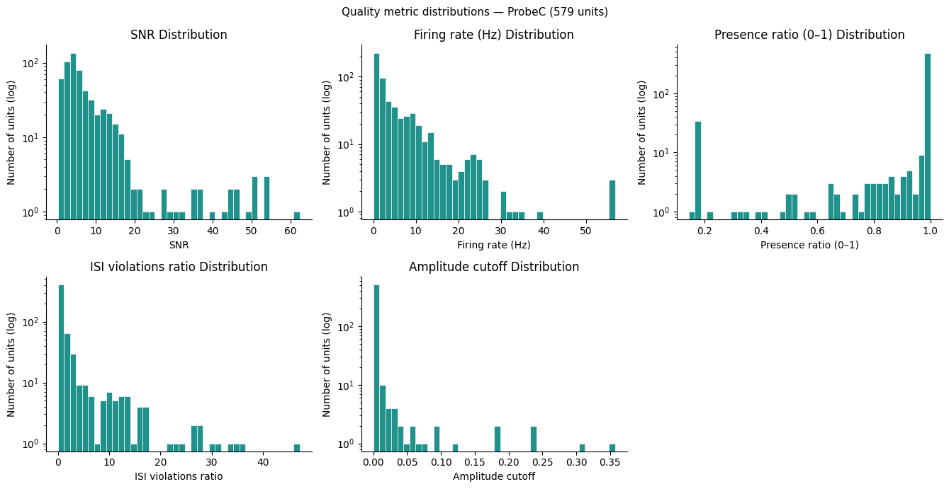
Quality filtering — apply five waveform and stability metrics (
snr,firing_rate,presence_ratio,isi_violations_ratio,amplitude_cutoff) to discard multi-unit noise and unstable isolations. Among the thresholds used, those forpresence_ratio,isi_violations_ratio, andamplitude_cutoffare conventional within the Allen Institute and roughly match what a human curator would select. The thresholds forsnrandfiring_rateare chosen arbitrarily and may be adjusted based on the distributions plotted below.Depth sorting — reorder the passing units by
estimated_y, an estimate of each unit’s position along the probe shank derived from the spike waveform centre-of-mass. This gives depth-ordered rows in all heatmaps and rasters. True Allen CCF coordinates are not yet available (see Section 4).
Note:
nwb.units.to_dataframe()can be memory-intensive for sessions with many units. The cells below access quality metrics column-by-column to avoid loading all data at once.
n_units_total = len(nwb.units)
print(f"Total units in this session: {n_units_total}")
print(f"Unit table columns: {list(nwb.units.colnames)}")
print()

# --- Step 1: Probe selection ---
# Choose which probe to analyse before inspecting quality metrics so that
# the distributions shown below reflect only that probe's recording environment.
# Set to None to include all probes.
PROBE_FILTER = "ProbeC"   # <-- EDIT THIS (e.g. "ProbeA", "ProbeB", ..., or None)


def get_unit_probe(unit_idx):
    """Return the probe name (e.g. 'ProbeC') for a given unit index."""
    if 'device_name' in nwb.units.colnames:
        return nwb.units['device_name'][unit_idx]
    return None


print(f"Available probes: {sorted(set(nwb.electrode_groups.keys()))}")

if PROBE_FILTER is not None:
    probe_unit_indices = [i for i in range(n_units_total) if get_unit_probe(i) == PROBE_FILTER]
    print(f"Probe '{PROBE_FILTER}': {len(probe_unit_indices)} / {n_units_total} units selected.")
else:
    probe_unit_indices = list(range(n_units_total))
    print(f"No probe filter — using all {n_units_total} units.")
Total units in this session: 3749
Unit table columns: ['spike_times', 'electrodes', 'waveform_mean', 'waveform_sd', 'unit_name', 'peak_trough_ratio', 'isi_violations_ratio', 'amplitude_cv_range', 'firing_rate', 'drift_ptp', 'silhouette', 'num_positive_peaks', 'decoder_label', 'nn_miss_rate', 'repolarization_slope', 'amplitude_cutoff', 'drift_mad', 'device_name', 'velocity_below', 'isi_violations_count', 'half_width', 'num_negative_peaks', 'presence_ratio', 'shank', 'spread', 'amplitude', 'estimated_z', 'exp_decay', 'estimated_y', 'l_ratio', 'decoder_probability', 'rp_violations', 'estimated_x', 'recovery_slope', 'sync_spike_4', 'depth', 'amplitude_cv_median', 'sync_spike_8', 'sliding_rp_violation', 'nn_hit_rate', 'drift_std', 'isolation_distance', 'extremum_channel_index', 'snr', 'num_spikes', 'rp_contamination', 'ks_unit_id', 'firing_range', 'original_cluster_id', 'amplitude_median', 'velocity_above', 'peak_to_valley', 'default_qc', 'd_prime', 'sync_spike_2']

Available probes: ['ProbeA', 'ProbeB', 'ProbeC', 'ProbeD', 'ProbeE', 'ProbeF']
Probe 'ProbeC': 579 / 3749 units selected.
# --- Step 2a: Load quality metrics for the selected probe's units ---
# Loading per-probe (not all units) keeps distributions focused on the
# recording environment you are actually analysing.
def _load_col(colname):
    if colname in nwb.units.colnames:
        return np.array([nwb.units[colname][i] for i in probe_unit_indices])
    return None

snr_values       = _load_col('snr')
fr_values        = _load_col('firing_rate')
presence_values  = _load_col('presence_ratio')
isi_values       = _load_col('isi_violations_ratio')
amp_cut_values   = _load_col('amplitude_cutoff')

print(f"SNR range:                {np.nanmin(snr_values):.2f} – {np.nanmax(snr_values):.2f}")
if fr_values       is not None: print(f"Firing rate range:        {np.nanmin(fr_values):.2f} – {np.nanmax(fr_values):.2f} Hz")
if presence_values is not None: print(f"Presence ratio range:     {np.nanmin(presence_values):.2f} – {np.nanmax(presence_values):.2f}")
if isi_values      is not None: print(f"ISI violations ratio:     {np.nanmin(isi_values):.4f} – {np.nanmax(isi_values):.4f}")
if amp_cut_values  is not None: print(f"Amplitude cutoff range:   {np.nanmin(amp_cut_values):.4f} – {np.nanmax(amp_cut_values):.4f}")

# --- Step 2b: Plot quality metric distributions ---
metrics = [
    (snr_values,      "SNR"),
    (fr_values,       "Firing rate (Hz)"),
    (presence_values, "Presence ratio (0–1)"),
    (isi_values,      "ISI violations ratio"),
    (amp_cut_values,  "Amplitude cutoff"),
]
metrics = [(v, l) for v, l in metrics if v is not None]

MAX_COLS = 3
n_plots  = len(metrics)
n_cols   = min(n_plots, MAX_COLS)
n_rows   = math.ceil(n_plots / n_cols)

fig, axes = plt.subplots(n_rows, n_cols, figsize=(4.5 * n_cols, 3.5 * n_rows))
axes = np.array(axes).reshape(-1)

for i, (vals, xlabel) in enumerate(metrics):
    ax = axes[i]
    vals_clean = vals[~np.isnan(vals)]
    ax.hist(vals_clean, bins=40, color=plt.cm.viridis(0.5), edgecolor='white', linewidth=0.5)
    ax.set_yscale('log')
    ax.set_xlabel(xlabel)
    ax.set_ylabel("Number of units (log)")
    ax.set_title(xlabel + " Distribution")
    ax.spines['top'].set_visible(False)
    ax.spines['right'].set_visible(False)

for j in range(n_plots, len(axes)):
    axes[j].set_visible(False)

fig.suptitle(
    f"Quality metric distributions — {PROBE_FILTER if PROBE_FILTER else 'all probes'} "
    f"({len(probe_unit_indices)} units)",
    fontsize=11)
plt.tight_layout()
plt.show()
SNR range:                0.24 – 62.37
Firing rate range:        0.01 – 56.86 Hz
Presence ratio range:     0.14 – 1.00
ISI violations ratio:     0.0000 – 47.1294
Amplitude cutoff range:   0.0000 – 0.3573
# --- Step 2c: Apply quality thresholds ---
# Adjust thresholds based on the distributions plotted above.
# Metric arrays are indexed locally (position 0 = first unit in probe_unit_indices).
SNR_THRESHOLD        = 4.0   # keep units with SNR above this
FR_MIN               = 0.1   # Hz — discard near-silent units
PRESENCE_MIN         = 0.9   # fraction of session — discard units that disappear mid-session
ISI_MAX              = 0.5   # ISI violation rate — discard heavily contaminated units
AMPLITUDE_CUTOFF_MAX = 0.1   # est. fraction of spikes below threshold — discard poorly detected units

selected_unit_indices = []
for local_i, abs_i in enumerate(probe_unit_indices):
    if snr_values[local_i] <= SNR_THRESHOLD:
        continue
    if fr_values is not None and fr_values[local_i] < FR_MIN:
        continue
    if presence_values is not None and presence_values[local_i] < PRESENCE_MIN:
        continue
    if isi_values is not None and isi_values[local_i] > ISI_MAX:
        continue
    if amp_cut_values is not None and amp_cut_values[local_i] > AMPLITUDE_CUTOFF_MAX:
        continue
    selected_unit_indices.append(abs_i)

n_probe = len(probe_unit_indices)
print(f"SNR > {SNR_THRESHOLD}:                         {sum(snr_values > SNR_THRESHOLD)} / {n_probe}")
if fr_values       is not None: print(f"  + firing rate >= {FR_MIN} Hz:          {sum((snr_values > SNR_THRESHOLD) & (fr_values >= FR_MIN))} remaining")
if presence_values is not None: print(f"  + presence ratio >= {PRESENCE_MIN}:       {sum((snr_values > SNR_THRESHOLD) & (fr_values >= FR_MIN) & (presence_values >= PRESENCE_MIN))} remaining")
if isi_values      is not None: print(f"  + ISI violations <= {ISI_MAX}:         {sum((snr_values > SNR_THRESHOLD) & (fr_values >= FR_MIN) & (presence_values >= PRESENCE_MIN) & (isi_values <= ISI_MAX))} remaining")
if amp_cut_values  is not None: print(f"  + amplitude cutoff <= {AMPLITUDE_CUTOFF_MAX}:       {sum((snr_values > SNR_THRESHOLD) & (fr_values >= FR_MIN) & (presence_values >= PRESENCE_MIN) & (isi_values <= ISI_MAX) & (amp_cut_values <= AMPLITUDE_CUTOFF_MAX))} remaining")

print(f"\nUnits passing quality filters: {len(selected_unit_indices)} / {n_probe}")
SNR > 4.0:                         354 / 579
  + firing rate >= 0.1 Hz:          323 remaining
  + presence ratio >= 0.9:       278 remaining
  + ISI violations <= 0.5:         178 remaining
  + amplitude cutoff <= 0.1:       178 remaining

Units passing quality filters: 178 / 579
# --- Step 3: Load spike times and sort by depth ---
# Load spike times only for the quality-filtered units.
print("Loading spike times...")
spike_times_list = [np.array(nwb.units['spike_times'][i]) for i in selected_unit_indices]
print(f"Loaded {len(spike_times_list)} units.")

# Reorder by estimated_y (superficial → deep) so all downstream cells
# (raster, heatmaps, PSTH) use a consistent depth ordering.
# Units missing estimated_y (NaN / Inf) are placed at the end.
if 'estimated_y' in nwb.units.colnames:
    _est_y     = np.array([nwb.units['estimated_y'][i] for i in selected_unit_indices],
                           dtype=float)
    _depth_ord = np.argsort(np.where(np.isfinite(_est_y), _est_y, np.inf))
    selected_unit_indices = [selected_unit_indices[j] for j in _depth_ord]
    spike_times_list  = [spike_times_list[j]  for j in _depth_ord]
    print(f"Units sorted by estimated_y (superficial → deep).")
else:
    print("'estimated_y' not available — units kept in natural order.")

# Show a few example units (in depth order)
for k, idx in enumerate(selected_unit_indices[:5]):
    n_spk = len(spike_times_list[k])
    dur   = spike_times_list[k][-1] - spike_times_list[k][0] if n_spk > 1 else 0
    print(f"  Unit {idx:4d} ({get_unit_probe(idx)}): {n_spk:6d} spikes,  "
          f"mean FR = {n_spk/dur:.2f} Hz" if dur > 0 else f"  Unit {idx:4d}: {n_spk} spikes")
Loading spike times...
Loaded 178 units.
Units sorted by estimated_y (superficial → deep).
  Unit 1303 (ProbeC): 117308 spikes,  mean FR = 21.69 Hz
  Unit 1304 (ProbeC):  10196 spikes,  mean FR = 1.89 Hz
  Unit 1317 (ProbeC):  17366 spikes,  mean FR = 3.21 Hz
  Unit 1316 (ProbeC):  18604 spikes,  mean FR = 3.44 Hz
  Unit 1315 (ProbeC):  41752 spikes,  mean FR = 7.72 Hz
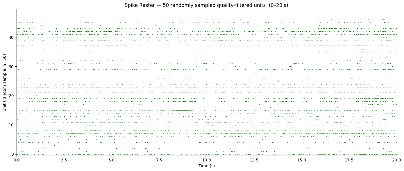
# Spike raster: randomly sample up to RASTER_MAX_UNITS units, show RASTER_DUR seconds.
# Random sampling preserves the natural mix of firing rates across the population.
RASTER_MAX_UNITS = 50
RASTER_START     = 0.0   # seconds after first spike time to begin
RASTER_DUR       = 20.0  # seconds to display

t_lo = float(spike_times_list[0][0]) + RASTER_START
t_hi = t_lo + RASTER_DUR

rng_units = np.random.default_rng(seed=0)
n_show    = min(RASTER_MAX_UNITS, len(spike_times_list))
unit_idx  = np.sort(rng_units.choice(len(spike_times_list), size=n_show, replace=False))

fig, ax = plt.subplots(figsize=(14, max(4, n_show * 0.12)))

for row, ui in enumerate(unit_idx):
    spk  = spike_times_list[ui]
    mask = (spk >= t_lo) & (spk < t_hi)
    ax.scatter(
        spk[mask] - t_lo,
        np.full(mask.sum(), row),
        s=2, marker="|", linewidths=0.7,
        color="green",
    )

ax.set_xlim(0, RASTER_DUR)
ax.set_ylim(-0.5, n_show - 0.5)
ax.set_xlabel("Time (s)")
ax.set_ylabel(f"Unit (random sample, n={n_show})")
ax.set_title(
    f"Spike Raster — {n_show} randomly sampled quality-filtered units  "
    f"({RASTER_START:.0f}–{RASTER_START + RASTER_DUR:.0f} s)"
)
ax.spines["top"].set_visible(False)
ax.spines["right"].set_visible(False)
plt.tight_layout()
plt.show()
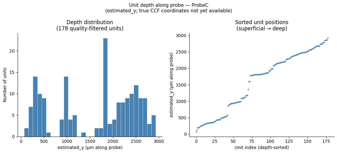
Sorting Units by Depth
Each spike-sorted unit has an estimated_y column in the units table that reports its estimated position along the probe shank in microns. This value is derived from the centre-of-mass of the spike waveform across channels and provides a relative depth ordering within the probe — shallower units appear at low estimated_y values, deeper units at higher values.
Note: As described in the electrodes table section above, true Allen CCF coordinates (
x,y,z) and brain-area annotations are not yet available for Dandiset 001637 — those fields will be populated in a future re-release once SmartSPIM light-sheet processing is complete.estimated_yis therefore the best available proxy for cortical depth at this time and should be interpreted as a relative rather than absolute anatomical position.
# Visualise the depth distribution of the selected units.
# selected_unit_indices / spike_times_list are already sorted by estimated_y (see cell above).
if 'estimated_y' in nwb.units.colnames:
    est_y_all   = np.array([nwb.units['estimated_y'][i] for i in selected_unit_indices],
                            dtype=float)
    valid_mask  = np.isfinite(est_y_all)
    est_y_valid = est_y_all[valid_mask]

    print(f"estimated_y: {valid_mask.sum()} / {len(selected_unit_indices)} units have valid values")
    print(f"Range: {est_y_valid.min():.1f} – {est_y_valid.max():.1f} µm")

    fig, axes = plt.subplots(1, 2, figsize=(11, 5))

    # Left panel — histogram of estimated_y distribution
    ax_hist = axes[0]
    ax_hist.hist(est_y_valid, bins=30, color="steelblue", edgecolor="white", linewidth=0.4)
    ax_hist.set_xlabel("estimated_y (µm along probe)")
    ax_hist.set_ylabel("Number of units")
    ax_hist.set_title(f"Depth distribution\n({len(est_y_valid)} quality-filtered units)")
    ax_hist.spines["top"].set_visible(False)
    ax_hist.spines["right"].set_visible(False)

    # Right panel — unit index (0 = shallowest) vs estimated_y
    ax_sc = axes[1]
    ax_sc.scatter(np.arange(len(est_y_all)), est_y_all,
                  s=6, c="steelblue", alpha=0.7)
    ax_sc.set_xlabel("Unit index (depth-sorted)")
    ax_sc.set_ylabel("estimated_y (µm along probe)")
    ax_sc.set_title("Sorted unit positions\n(superficial → deep)")
    ax_sc.spines["top"].set_visible(False)
    ax_sc.spines["right"].set_visible(False)

    fig.suptitle(
        f"Unit depth along probe — {PROBE_FILTER if PROBE_FILTER else 'all probes'}\n"
        "(estimated_y; true CCF coordinates not yet available)",
        fontsize=11)
    plt.tight_layout()
    plt.show()
else:
    print("'estimated_y' column not found in nwb.units — skipping depth plot.")
    print(f"Available unit columns: {list(nwb.units.colnames)}")
estimated_y: 178 / 178 units have valid values
Range: 68.8 – 2931.1 µm
6. Behavioral Data: Running and Eye Tracking
As in the Mesoscope dataset, the Neuropixels sessions include two behavioral streams:
Running wheel rotation — stored as raw cumulative rotation in
nwb.acquisition["raw_running_wheel_rotation"]. Unlike the ophys NWB, no pre-computed speed is available; we derive it by taking the numerical gradient of the cumulative rotation with respect to the timestamp vector.Eye tracking — pupil area from
nwb.processing['eye_tracking']['pupil'], same path as in the Mesoscope NWB.
Running strongly modulates neural activity in visual cortex (locomotion gain effects), and pupil area is a proxy for arousal/brain state.
The behavioral overview plot below displays the first 600 s of the session. Each signal is independently zeroed to its own first timestamp, so the two subplots are not perfectly time-aligned with one another — they share the same x-axis range but are on independent recording clocks. See Section 9 for proper interpolation onto a shared time axis.
# --- Running wheel (raw rotation → speed) ---
wheel = nwb.acquisition["raw_running_wheel_rotation"]
wheel_rotation   = np.array(wheel.data)
wheel_timestamps = np.array(wheel.timestamps)

# Compute angular velocity (deg/s or cm/s depending on unit) via numerical gradient
# np.gradient handles unequal spacing and avoids boundary artifacts
running_speed_data       = np.gradient(np.cumsum(wheel_rotation), wheel_timestamps)
running_speed_timestamps = wheel_timestamps

print(f"Running wheel: {len(wheel_rotation)} samples, "
      f"duration {wheel_timestamps[-1] - wheel_timestamps[0]:.1f} s")
print(f"Derived running speed: min={running_speed_data.min():.1f},  "
      f"max={running_speed_data.max():.1f},  "
      f"units: {wheel.unit if hasattr(wheel, 'unit') else 'unknown'}")
Running wheel: 265441 samples, duration 4427.7 s
Derived running speed: min=-85.1, max=97.5, units: radians
# --- Eye tracking (pupil area) ---
pupil = nwb.processing['eye_tracking']['pupil']
eye_tracking_area       = np.array(pupil['area'])
eye_tracking_timestamps = np.array(pupil['timestamps'])

print(f"Eye tracking (pupil area): {len(eye_tracking_area)} samples, "
      f"duration {eye_tracking_timestamps[-1] - eye_tracking_timestamps[0]:.1f} s")
Eye tracking (pupil area): 324908 samples, duration 5415.0 s
BEHAV_WINDOW = (0, 600)  # seconds to display

fig, axes = plt.subplots(2, 1, figsize=(14, 6), sharex=True)

# NOTE: each signal is zeroed to its *own* first timestamp, not a common session
# clock.  The two subplots therefore share the same x-axis range (0–600 s) but
# are on independent time axes and are not perfectly aligned with each other.
# See Section 9 for proper interpolation onto a single shared time axis.

# --- Running speed ---
rs_t    = running_speed_timestamps - running_speed_timestamps[0]
mask_rs = (rs_t >= BEHAV_WINDOW[0]) & (rs_t <= BEHAV_WINDOW[1])
axes[0].plot(rs_t[mask_rs], running_speed_data[mask_rs], lw=0.7, color="darkorange")
axes[0].set_ylabel("Running speed\n(wheel units/s)")
axes[0].set_title("Running Speed")
axes[0].spines["top"].set_visible(False)
axes[0].spines["right"].set_visible(False)

# --- Eye tracking (pupil area) ---
et_t    = eye_tracking_timestamps - eye_tracking_timestamps[0]
mask_et = (et_t >= BEHAV_WINDOW[0]) & (et_t <= BEHAV_WINDOW[1])
axes[1].plot(et_t[mask_et], eye_tracking_area[mask_et], lw=0.7, color="purple")
axes[1].set_ylabel("Pupil area\n(pixels²)")
axes[1].set_title("Eye Tracking (Pupil Area)")
axes[1].set_xlabel("Time from session start (s)")
axes[1].spines["top"].set_visible(False)
axes[1].spines["right"].set_visible(False)

fig.suptitle("Behavioral Overview (first 600 s)", fontsize=13)
plt.tight_layout()
plt.show()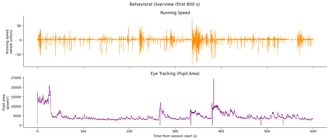
7. Stimulus Tables and Block Structure
All stimulus information is stored in nwb.intervals. Each table row represents one stimulus presentation with columns including:
start_time,stop_time— onset and offset in secondsTrialType— the category of the presentation (standard vs. oddball)Grating properties:
orientation,temporal_frequency,spatial_frequency,contrast
Stimulus Table Catalogue
Every session contains all four control blocks plus exactly one mismatch (oddball) block — the specific oddball type identifies the experimental paradigm for that session. Each control block is paired with its corresponding mismatch block as a matched baseline.
| Oddball block | Paired control | Paradigm | What the mouse predicts |
|---|---|---|---|
Standard mismatch block_presentations | Control block 1_presentations | Standard oddball | Identity of a repeated grating |
Sequence mismatch block_presentations | Control block 2_presentations | Sequence mismatch | Position of a grating within a fixed ABCD sequence |
Duration mismatch block_presentations | Control block 3_presentations | Temporal jitter | Regularity of inter-stimulus timing |
Sensory-motor mismatch block_presentations | Control block 4_presentations | Sensorimotor mismatch | Visual flow coupled to the animal’s running |
Additional tables present in all or most sessions:
| Table | Contents |
|---|---|
spontaneous_presentations | Spontaneous activity epoch (no stimulus) |
RF mapping_presentations | Receptive-field mapping stimuli |
Zebra_presentations | Zebra noise stimulus — dynamic stripes that vary randomly in orientation, width, eccentricity, direction, and speed |
40 hz pulse train_presentations | Optogenetic tagging — 40 Hz pulse train |
5 hz pulse train_presentations | Optogenetic tagging — 5 Hz pulse train |
raised_cosine_presentations | Optogenetic tagging — raised-cosine waveform |
Sequence Mismatch Stimulus Design
In this sequence mismatch session, stimuli are presented in repeating 4-element sequences (ABCD). Occasional oddballs replace the 3rd position (C) with an unexpected grating. The TrialType column distinguishes:
Standard sequence elements — the expected grating at each position
Oddball insertions — the unexpected 3rd-position grating
The epoch structure timeline below visualizes the session’s block organization.
# List all available stimulus tables
stim_table_names = list(nwb.intervals.keys())
print("Stimulus tables in this NWB:")
for name in stim_table_names:
    tbl = nwb.intervals[name]
    print(f"  {name!r:60s}  ({len(tbl)} rows)")
Stimulus tables in this NWB:
'40 hz pulse train_presentations' (150 rows)
'5 hz pulse train_presentations' (148 rows)
'Control block 1_presentations' (1088 rows)
'Control block 2_presentations' (1120 rows)
'Control block 3_presentations' (368 rows)
'Control block 4_presentations' (11520 rows)
'RF mapping_presentations' (1215 rows)
'Sequence mismatch block_presentations' (6240 rows)
'Zebra_presentations' (18000 rows)
'raised_cosine_presentations' (149 rows)
'spontaneous_presentations' (4 rows)
# Inspect this session's oddball stimulus table
stim_name = "Sequence mismatch block_presentations"
stim_table = nwb.intervals[stim_name]

stim_df = stim_table.to_dataframe()
print(f"Table: {stim_name!r}")
print(f"Columns: {list(stim_table.colnames)}")
print(f"TrialTypes: {set(stim_df['TrialType'])}")
stim_table[:10]
Table: 'Sequence mismatch block_presentations'
Columns: ['start_time', 'stop_time', 'stim_name', 'stim_type', 'stim_block', 'Orientation', 'SpatialFrequency', 'TemporalFrequency', 'contrast', 'phase', 'DiameterX', 'DiameterY', 'X', 'Y', 'Duration', 'Delay', 'BlockNumber', 'BlockLabel', 'TrialNumber', 'SequenceNumber', 'TrialInSequence', 'TrialType', 'BlockType', 'stim_index', 'timeseries']
TrialTypes: {'halt', 'orientation_45', 'omission', 'standard', 'orientation_90', 'sequence_omission'}
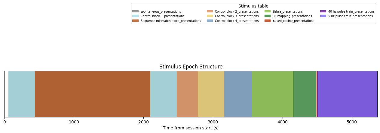
Epoch Structure Timeline
Here we extract epochs — contiguous intervals during which the same stimulus context is shown — and visualize them as a colored timeline.
def extract_epochs(stim_name, stim_table, epochs):
    """Extract contiguous stimulus epochs from a presentation table."""
    block_key = None
    for candidate in ["stim_block", "stimulus_block", "stimulus_type", "TrialType"]:
        if candidate in stim_table.colnames:
            block_key = candidate
            break

    if block_key is None:
        epoch_start = stim_table.start_time[0]
        epoch_stop  = stim_table.stop_time[-1]
        epochs.append((stim_name, stim_name, epoch_start, epoch_stop))
        return epochs

    epoch_start = stim_table.start_time[0]
    epoch_stop  = stim_table.stop_time[0]

    for i in range(len(stim_table)):
        this_block = stim_table[block_key][i]
        if i + 1 >= len(stim_table):
            epochs.append((stim_name, this_block, epoch_start, epoch_stop))
            break
        next_block = stim_table[block_key][i + 1]
        if next_block == this_block:
            epoch_stop = stim_table.stop_time[i + 1]
        else:
            epochs.append((stim_name, this_block, epoch_start, epoch_stop))
            epoch_start = stim_table.start_time[i + 1]
            epoch_stop  = stim_table.stop_time[i + 1]

    return epochs


epochs = []
for sn in stim_table_names:
    try:
        epochs = extract_epochs(sn, nwb.intervals[sn], epochs)
    except Exception:
        continue

epochs.sort(key=lambda x: x[2])
print(f"Total epochs found: {len(epochs)}")
for ep in epochs[:20]:
    print(f"  {ep[0]!s:<40}  {ep[2]:.1f} – {ep[3]:.1f} s  ({ep[3]-ep[2]:.1f} s)")
Total epochs found: 12
spontaneous_presentations 56.5 – 4158.6 s (4102.1 s)
Control block 1_presentations 56.5 – 437.0 s (380.5 s)
Sequence mismatch block_presentations 437.0 – 2099.7 s (1662.8 s)
Control block 1_presentations 2100.1 – 2480.8 s (380.8 s)
Control block 2_presentations 2480.8 – 2779.3 s (298.5 s)
Control block 3_presentations 2780.2 – 3164.1 s (383.9 s)
Control block 4_presentations 3164.1 – 3558.6 s (394.5 s)
Zebra_presentations 3558.6 – 4158.6 s (600.0 s)
RF mapping_presentations 4158.6 – 4482.4 s (323.8 s)
raised_cosine_presentations 4491.7 – 5352.4 s (860.7 s)
40 hz pulse train_presentations 4497.4 – 5360.1 s (862.7 s)
5 hz pulse train_presentations 4511.4 – 5363.9 s (852.5 s)
unique_stim_names = list({ep[0] for ep in epochs})

# Fixed color map — one visually distinct color per stimulus table.
# Mismatch/oddball tables use dark bold colors; paired controls use a lighter version.
STIM_COLORS = {
    # Oddball epochs (dark / bold)
    "Standard mismatch block_presentations":      "#4FC3CF",  # aquamarine
    "Sequence mismatch block_presentations":      "#B5541A",  # burnt orange
    "Duration mismatch block_presentations":      "#C8941A",  # goldenrod
    "Sensory-motor mismatch block_presentations": "#1B3A7A",  # navy blue
    # Paired control epochs (lighter version of the paired oddball)
    "Control block 1_presentations":              "#A8DDE6",  # light aquamarine (→ Standard)
    "Control block 2_presentations":              "#E0905E",  # light orange   (→ Sequence)
    "Control block 3_presentations":              "#EDD070",  # light goldenrod (→ Duration)
    "Control block 4_presentations":              "#7A9FC2",  # light navy     (→ Motor)
    # Other epochs
    "spontaneous_presentations":                  "#808080",  # grey
    "RF mapping_presentations":                   "#2E7D32",  # dark forest green
    "Zebra_presentations":                        "#8BC34A",  # lime / yellow-green
    "40 hz pulse train_presentations":            "#6A1B9A",  # deep indigo-purple
    "5 hz pulse train_presentations":             "#7B68EE",  # periwinkle/lavender
    "raised_cosine_presentations":                "#BF360C",  # deep brick red
}
# Fall back to neutral grey for any table not listed above.
color_map = {name: STIM_COLORS.get(name, "#999999") for name in unique_stim_names}

session_end = max(ep[3] for ep in epochs)

fig, ax = plt.subplots(figsize=(16, 2))

legend_handles = {}
for ep in epochs:
    stim_name_ep, block_id, t_start, t_stop = ep
    color = color_map[stim_name_ep]
    patch = ax.axvspan(t_start, t_stop, color=color, alpha=0.8)
    if stim_name_ep not in legend_handles:
        legend_handles[stim_name_ep] = patch

ax.set_xlim(0, session_end)
ax.set_ylim(0, 1)
ax.set_yticks([])
ax.set_xlabel("Time from session start (s)")
ax.set_title("Stimulus Epoch Structure")
ax.legend(
    legend_handles.values(), legend_handles.keys(),
    loc="upper right", bbox_to_anchor=(1, 2.5),
    fontsize=7, ncols=4, title="Stimulus table"
)
plt.tight_layout()
plt.show()
8. Selecting Oddball (Mismatch) Stimulus Times
For the predictive processing analyses, the key events are the oddball presentations — the rare stimuli that violate the established sequential prediction. The TrialType column in the sequence mismatch table distinguishes the 3rd-position standard presentations from the oddball insertions at that position.
Set ODDBALL_TYPE and STANDARD_TYPE to the values printed by the exploratory cell below.
# Select the sequence mismatch stimulus table (skip spontaneous)
TYPE_COL = "TrialType"

non_spontaneous = [n for n in stim_table_names if "spontaneous" not in n.lower()]
# Prefer the sequence mismatch table if present
seq_tables = [n for n in non_spontaneous if "sequence" in n.lower()]
STIM_TABLE_NAME = seq_tables[0] if seq_tables else non_spontaneous[0]
stim_df = nwb.intervals[STIM_TABLE_NAME].to_dataframe()

print(f"Using stimulus table: {STIM_TABLE_NAME!r}")
print(f"Using type column:    {TYPE_COL!r}")
print(f"\nAvailable TrialTypes: {sorted(stim_df[TYPE_COL].unique().tolist())}")
Using stimulus table: 'Sequence mismatch block_presentations'
Using type column: 'TrialType'
Available TrialTypes: ['halt', 'omission', 'orientation_45', 'orientation_90', 'sequence_omission', 'standard']
# --- Choose the oddball and standard trial types ---
# Set ODDBALL_TYPE to one of the values printed above.
# Available types for this session:
#   'orientation_45'    — unexpected orientation (45°) at position 3  (n=35)
#   'orientation_90'    — unexpected orientation (90°) at position 3  (n=35)
#   'halt'              — motion halt deviant at position 3            (n=35)
#   'omission'          — stimulus omission at position 3              (n=35)
#   'sequence_omission' — omission of a 5th "ghost" position (n=1248); no position-matched standard exists
#   'standard'          — expected sequence elements at positions 1–4  (n=4852)
ODDBALL_TYPE  = "omission"      # <-- EDIT THIS to select a different deviant type
STANDARD_TYPE = "standard"

# For oddballs at position 3 (orientation_45/90, halt, omission), filter standards
# to the same sequence position for a matched comparison.
# For sequence_omission (position 5), no position-5 standard exists — use all standards.
# NOTE: TrialInSequence is stored as object dtype with string values ('1.0','2.0',...)
POSITION_MATCHED_TYPES = {"orientation_45", "orientation_90", "halt", "omission"}
STANDARD_POSITION = "3.0"  # string value in TrialInSequence column

if ODDBALL_TYPE in stim_df[TYPE_COL].values:
    oddball_times = stim_df.loc[stim_df[TYPE_COL] == ODDBALL_TYPE, "start_time"].values
    print(f"Found {len(oddball_times)} presentations of '{ODDBALL_TYPE}'")
else:
    print(f"'{ODDBALL_TYPE}' not found. Available: {sorted(stim_df[TYPE_COL].unique().tolist())}")
    oddball_times = np.array([])

if STANDARD_TYPE in stim_df[TYPE_COL].values:
    std_mask = stim_df[TYPE_COL] == STANDARD_TYPE
    if ODDBALL_TYPE in POSITION_MATCHED_TYPES and "TrialInSequence" in stim_df.columns:
        std_mask = std_mask & (stim_df["TrialInSequence"] == STANDARD_POSITION)
        print(f"Filtering standards to position {STANDARD_POSITION} (position-matched comparison)")
    else:
        print(f"Using all standard trials (no position filter — '{ODDBALL_TYPE}' is at position 5)")
    standard_times = stim_df.loc[std_mask, "start_time"].values
    print(f"Using {len(standard_times)} '{STANDARD_TYPE}' presentations for comparison.")
else:
    print(f"'{STANDARD_TYPE}' not found. Available: {sorted(stim_df[TYPE_COL].unique().tolist())}")
    standard_times = np.array([])
Found 35 presentations of 'omission'
Filtering standards to position 3.0 (position-matched comparison)
Using 1108 'standard' presentations for comparison.
9. Aligning Behavioral Signals to a Common Time Axis
Running speed and eye tracking are recorded at different sampling rates and stored with independent timestamp vectors. We interpolate both onto a single uniform time axis at 100 Hz — fast enough to capture behavioral dynamics while keeping array sizes manageable. This shared axis is used for all subsequent stimulus-aligned analyses.
INTERP_HZ = 100  # Hz for common time axis

t_start_global = 0.0
t_end_global   = max(float(running_speed_timestamps[-1]),
                     float(eye_tracking_timestamps[-1]))

time_axis = np.arange(t_start_global, t_end_global, step=1.0 / INTERP_HZ)

# Interpolate running speed
f_run = interpolate.interp1d(
    running_speed_timestamps, running_speed_data,
    kind="nearest", bounds_error=False, fill_value=0.0
)
interp_running = f_run(time_axis)

# Interpolate pupil area
f_eye = interpolate.interp1d(
    eye_tracking_timestamps, eye_tracking_area,
    kind="nearest", bounds_error=False, fill_value=np.nan
)
interp_eye = f_eye(time_axis)

print(f"Common time axis: {len(time_axis)} samples at {INTERP_HZ} Hz ({time_axis[-1]:.1f} s)")
print(f"interp_running shape: {interp_running.shape}")
print(f"interp_eye shape:     {interp_eye.shape}")
Common time axis: 542981 samples at 100 Hz (5429.8 s)
interp_running shape: (542981,)
interp_eye shape: (542981,)
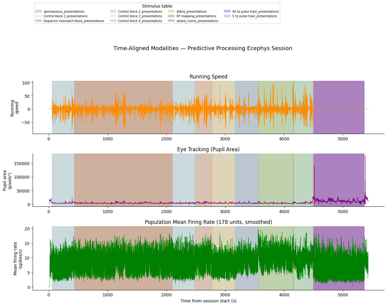
Aligned Overview Plot
With all signals on the same time axis we can overlay them with shared x-axis and add colored epoch bands to show the stimulus block structure. The third panel shows a coarse population-level spike rate (all good units summed and smoothed) for a quick neural overview.
Note that running speed is not recorded during the optotagging period because Bonsai, which drives the running wheel acquisition, is turned off for that part of the session.
# Build a coarse population spike-rate signal on the same time axis.
# Bin all spikes from quality units into 10 ms bins, then smooth with a Gaussian.
bin_size_pop  = 0.01  # 10 ms bins
pop_bin_edges = np.arange(0, time_axis[-1] + bin_size_pop, bin_size_pop)
pop_spike_counts = np.zeros(len(pop_bin_edges) - 1)
for spk in spike_times_list:
    counts, _ = np.histogram(spk, bins=pop_bin_edges)
    pop_spike_counts += counts

# Convert to firing rate (spikes/s) averaged over units, then smooth
pop_spike_rate  = pop_spike_counts / bin_size_pop / len(spike_times_list)
pop_spike_rate  = gaussian_filter1d(pop_spike_rate, sigma=5)  # ~50 ms Gaussian
pop_bin_centers = pop_bin_edges[:-1] + bin_size_pop / 2

print(f"Population spike rate: {len(pop_bin_centers)} bins, "
      f"peak = {pop_spike_rate.max():.2f} spikes/s")
Population spike rate: 542980 bins, peak = 19.74 spikes/s
def draw_epoch_bands(ax, epochs, view_start, view_end, cmap=None, alpha=0.30):
    """Shade each epoch as a semi-transparent colored band on the given axis.

    Uses ``ax.axvspan`` so the bands span the full y-axis without capturing
    the current ylim and without interfering with autoscaling.
    """
    if cmap is None:
        unique_labels = list({ep[0] for ep in epochs})
        tab_colors    = plt.cm.tab20(np.linspace(0, 1, len(unique_labels)))
        cmap          = dict(zip(unique_labels, tab_colors))

    legend_handles = {}
    for ep in epochs:
        stim_name_ep, _, t_s, t_e = ep
        if t_e < view_start or t_s > view_end:
            continue
        color = cmap.get(stim_name_ep, "gray")
        patch = ax.axvspan(
            max(t_s, view_start), min(t_e, view_end),
            color=color, alpha=alpha, zorder=0
        )
        legend_handles[stim_name_ep] = patch
    return legend_handles


VIEW_START = 0
VIEW_END   = int(time_axis[-1])

fig = plt.figure(figsize=(15, 9))
gs  = gridspec.GridSpec(3, 1, figure=fig, height_ratios=[1, 1, 1.2], hspace=0.35)

ax0 = fig.add_subplot(gs[0])
ax1 = fig.add_subplot(gs[1], sharex=ax0)
ax2 = fig.add_subplot(gs[2], sharex=ax0)

# --- Running speed ---
mask_rs = (time_axis >= VIEW_START) & (time_axis <= VIEW_END)
ax0.plot(time_axis[mask_rs], interp_running[mask_rs], lw=0.6, color="darkorange")
ax0.set_ylabel("Running\nspeed")
ax0.set_title("Running Speed")
ax0.spines["top"].set_visible(False); ax0.spines["right"].set_visible(False)
lh = draw_epoch_bands(ax0, epochs, VIEW_START, VIEW_END, cmap=color_map)

# --- Pupil area ---
ax1.plot(time_axis[mask_rs], interp_eye[mask_rs], lw=0.6, color="purple")
ax1.set_ylabel("Pupil area\n(pixels²)")
ax1.set_title("Eye Tracking (Pupil Area)")
ax1.spines["top"].set_visible(False); ax1.spines["right"].set_visible(False)
draw_epoch_bands(ax1, epochs, VIEW_START, VIEW_END, cmap=color_map)

# --- Population spike rate ---
mask_pop = (pop_bin_centers >= VIEW_START) & (pop_bin_centers <= VIEW_END)
ax2.plot(pop_bin_centers[mask_pop], pop_spike_rate[mask_pop], lw=0.6, color="green")
ax2.set_ylabel("Mean firing rate\n(spikes/s)")
ax2.set_title(f"Population Mean Firing Rate ({len(spike_times_list)} units, smoothed)")
ax2.set_xlabel("Time from session start (s)")
ax2.spines["top"].set_visible(False); ax2.spines["right"].set_visible(False)
draw_epoch_bands(ax2, epochs, VIEW_START, VIEW_END, cmap=color_map)

if lh:
    ax0.legend(
        lh.values(), lh.keys(),
        ncols=4, fontsize=7,
        loc="upper left", bbox_to_anchor=(0, 2.5),
        title="Stimulus table"
    )

fig.suptitle("Time-Aligned Modalities — Predictive Processing Ecephys Session",
             fontsize=13, y=1.01)
plt.tight_layout()
plt.show()
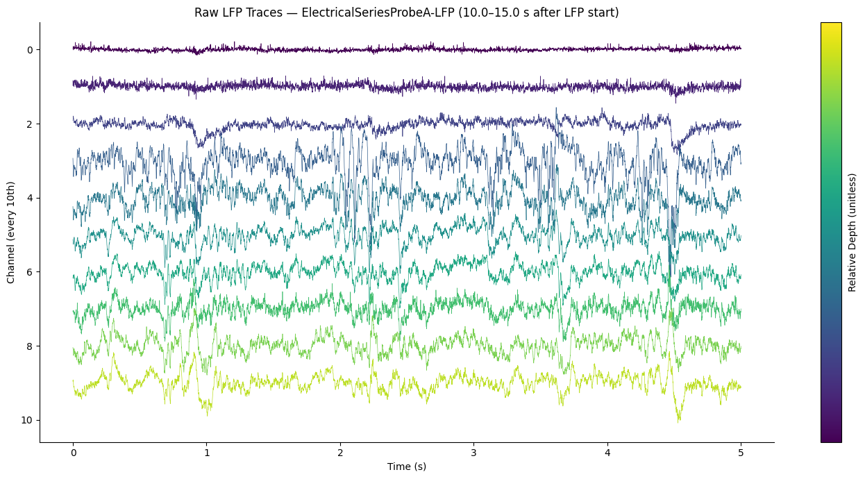
10. LFP Data
Local Field Potentials (LFP) are stored under nwb.processing['ecephys']['LFP'].electrical_series as a dictionary of ElectricalSeries objects, one per probe. The dictionary keys follow the pattern ElectricalSeriesProbeA-LFP, ElectricalSeriesProbeB-LFP, etc.
Each ElectricalSeries has:
.data— a 2D array of shape(n_timepoints, n_channels), sampled at ~1250 Hz.timestamps— the LFP time vector.electrodes— a reference table linking each column to the electrodes table
Performance note: LFP arrays are large. The cells below select one probe and a short time window to avoid loading the full dataset into memory. Adjust the probe and time window as needed for your analysis.
Note on superficial channels: The most superficial channels (low channel index / top of the raw trace plot) typically show a noisy, low-amplitude signal — these channels are outside the brain. Neuropixels probes extend beyond the brain surface at the insertion site, so the uppermost channels record ambient electrical noise rather than neural activity. Only channels below the brain surface show coherent LFP oscillations and stimulus-locked responses.
# Access LFP electrical series for all probes
lfp_series = nwb.processing['ecephys']['LFP'].electrical_series
print("LFP series keys:")
for key in lfp_series.keys():
    es = lfp_series[key]
    print(f"  {key}: shape {es.data.shape},  rate ~{1/np.median(np.diff(np.array(es.timestamps[:200]))):.0f} Hz")

# Select the first probe for visualization
LFP_PROBE_KEY = list(lfp_series.keys())[0]
lfp = lfp_series[LFP_PROBE_KEY]
lfp_timestamps = np.array(lfp.timestamps)

print(f"\nSelected probe: {LFP_PROBE_KEY}")
print(f"LFP shape: {lfp.data.shape}  (timepoints × channels)")
print(f"LFP duration: {lfp_timestamps[-1] - lfp_timestamps[0]:.1f} s")
LFP series keys:
ElectricalSeriesProbeA-LFP: shape (6761788, 96), rate ~1250 Hz
ElectricalSeriesProbeB-LFP: shape (6761786, 96), rate ~1250 Hz
ElectricalSeriesProbeC-LFP: shape (6761796, 96), rate ~1250 Hz
ElectricalSeriesProbeD-LFP: shape (6761775, 96), rate ~1250 Hz
ElectricalSeriesProbeE-LFP: shape (6761783, 96), rate ~1250 Hz
ElectricalSeriesProbeF-LFP: shape (6761779, 96), rate ~1250 Hz
Selected probe: ElectricalSeriesProbeA-LFP
LFP shape: (6761788, 96) (timepoints × channels)
LFP duration: 5409.4 s
# Plot a short snippet of raw LFP traces (first 5 s, select every 10th channel)
LFP_SNIPPET_START = 10.0   # seconds after LFP start (skip first ~10s of potential artefacts)
LFP_SNIPPET_DUR   = 5.0    # seconds to show
CHANNEL_STRIDE    = 10     # display every Nth channel

# lfp_timestamps are absolute session times — offset by the first timestamp
t0_idx = int(np.searchsorted(lfp_timestamps, lfp_timestamps[0] + LFP_SNIPPET_START))
t1_idx = int(np.searchsorted(lfp_timestamps, lfp_timestamps[0] + LFP_SNIPPET_START + LFP_SNIPPET_DUR))

# Load the snippet (timepoints × channels)
lfp_snippet = np.array(lfp.data[t0_idx:t1_idx, ::CHANNEL_STRIDE])
t_snip = lfp_timestamps[t0_idx:t1_idx] - lfp_timestamps[t0_idx]
n_ch_display = lfp_snippet.shape[1]

print(f"Snippet indices: {t0_idx} – {t1_idx}  ({lfp_snippet.shape[0]} timepoints × {n_ch_display} channels)")

fig, ax = plt.subplots(figsize=(14, 7))

# Normalize each channel and offset for display
scale = np.nanstd(lfp_snippet) * 4
for ch in range(n_ch_display):
    trace = lfp_snippet[:, ch] / (scale + 1e-12)
    ax.plot(t_snip, trace + ch, lw=0.5, color=plt.cm.viridis(ch / n_ch_display))

sm = plt.cm.ScalarMappable(cmap="viridis", norm=plt.Normalize(0, n_ch_display - 1))
sm.set_array([])
cb = plt.colorbar(sm, ax=ax, label="Relative Depth (unitless)") # depth is not known absolutely without CCF coordinates
cb.set_ticks([])

ax.invert_yaxis()
ax.set_xlabel("Time (s)")
ax.set_ylabel("Channel (every 10th)")
ax.set_title(f"Raw LFP Traces — {LFP_PROBE_KEY} "
             f"({LFP_SNIPPET_START}–{LFP_SNIPPET_START + LFP_SNIPPET_DUR} s after LFP start)")
ax.spines['top'].set_visible(False)
ax.spines['right'].set_visible(False)
plt.tight_layout()
plt.show()
Snippet indices: 12501 – 18751 (6250 timepoints × 10 channels)
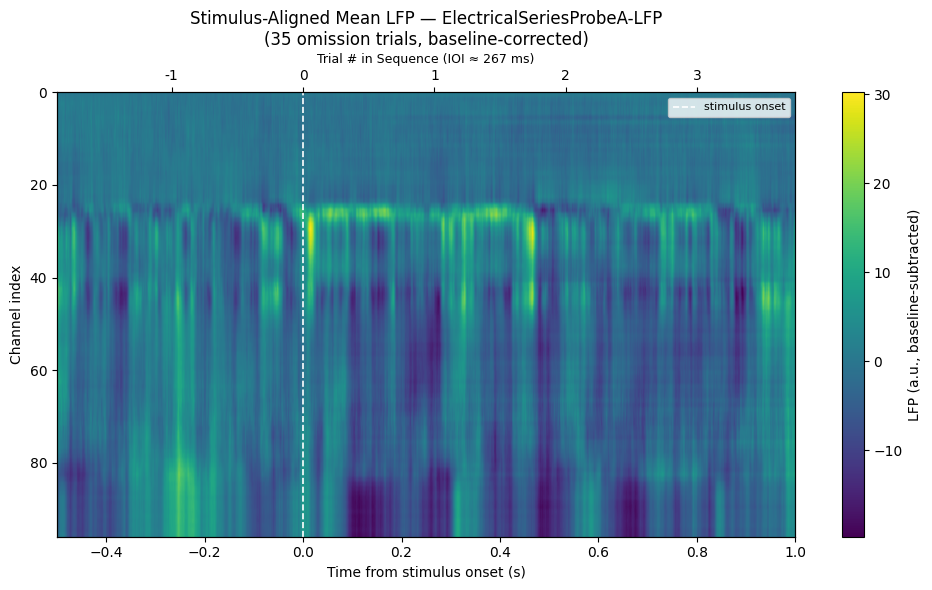
# Stimulus-aligned LFP heatmap across channels
# For each oddball trial, extract a window of LFP and average across trials.
LFP_WIN_PRE  = -0.5  # s before stimulus onset
LFP_WIN_POST =  1.0  # s after stimulus onset

if len(oddball_times) == 0:
    print("No oddball times available — skipping LFP alignment. Check ODDBALL_TYPE above.")
else:
    n_ch = lfp.data.shape[1]
    ch_indices = np.arange(0, n_ch)

    lfp_hz = 1 / np.median(np.diff(lfp_timestamps[:500]))
    lfp_win_len = int((LFP_WIN_POST - LFP_WIN_PRE) * lfp_hz)
    lfp_win_t   = np.linspace(LFP_WIN_PRE, LFP_WIN_POST, lfp_win_len)

    # Collect aligned LFP trials: (n_trials, n_channels, n_time)
    lfp_trials = []
    for t0 in oddball_times:
        i0 = int(np.searchsorted(lfp_timestamps, t0 + LFP_WIN_PRE))
        i1 = i0 + lfp_win_len
        if i0 >= 0 and i1 <= lfp.data.shape[0]:
            trial = np.array(lfp.data[i0:i1, :])  # (time, n_ch)
            # Baseline-subtract using the pre-stimulus window
            baseline_end = int(abs(LFP_WIN_PRE) * lfp_hz)
            trial = trial - trial[:baseline_end, :].mean(axis=0, keepdims=True)
            lfp_trials.append(trial.T)  # (n_ch, time)

    if lfp_trials:
        lfp_mean = np.mean(np.stack(lfp_trials, axis=0), axis=0)  # (n_ch, time)

        # Estimate inter-onset interval (IOI) from all consecutive stimulus onsets
        all_starts = np.sort(stim_df['start_time'].values)
        ioi = float(np.median(np.diff(all_starts)))

        fig, ax = plt.subplots(figsize=(10, 6))
        im = ax.imshow(
            lfp_mean,
            aspect="auto",
            extent=[LFP_WIN_PRE, LFP_WIN_POST, 0, lfp_mean.shape[0]],
            cmap="viridis",
            origin="lower",
        )
        ax.invert_yaxis()
        ax.axvline(0, color="white", lw=1.2, linestyle="--", label="stimulus onset")
        ax.set_xlabel("Time from stimulus onset (s)")
        ax.set_ylabel("Channel index")
        ax.set_title(f"Stimulus-Aligned Mean LFP — {LFP_PROBE_KEY}\n"
                     f"({len(lfp_trials)} {ODDBALL_TYPE} trials, baseline-corrected)")
        plt.colorbar(im, ax=ax, label="LFP (a.u., baseline-subtracted)")
        ax.legend(loc="upper right", fontsize=8)

        # Secondary x-axis at the top: numbered trial ticks at each IOI boundary
        ax_top = ax.twiny()
        ax_top.set_xlim(LFP_WIN_PRE, LFP_WIN_POST)
        n_back = int(np.floor(abs(LFP_WIN_PRE) / ioi))
        n_fwd  = int(np.floor(LFP_WIN_POST / ioi))
        trial_ticks  = [n * ioi for n in range(-n_back, n_fwd + 1)
                        if LFP_WIN_PRE <= n * ioi <= LFP_WIN_POST]
        trial_labels = [str(n) for n in range(-n_back, n_fwd + 1)
                        if LFP_WIN_PRE <= n * ioi <= LFP_WIN_POST]
        ax_top.set_xticks(trial_ticks)
        ax_top.set_xticklabels(trial_labels)
        ax_top.set_xlabel(f"Trial # in Sequence (IOI ≈ {ioi * 1000:.0f} ms)", fontsize=9)

        plt.tight_layout()
        plt.show()
    else:
        print("No valid LFP windows found for the selected oddball times.")
11. Spike Count Distributions
Three helper functions build the spike-rate summaries used throughout this section and the next:
get_trial_averaged_spike_rate— returns(n_units, n_bins)binned firing rates averaged across all trials for each unit; used for the heatmaps in Section 12.get_population_psth— returns(n_trials, n_bins)population-averaged firing rates, one trace per trial, used for ±SEM in Section 13.spike_counts_per_trial_unit— returns an(n_trials, n_units)integer matrix of total spike counts in the post-stimulus window, used for the distribution plots below.
Tip: Adjust
WINDOW_PRE,WINDOW_POST, andBIN_SIZEto control the analysis time window and temporal resolution. Smaller bins give finer resolution but noisier estimates; typical values are 5–25 ms.
The distribution plots below show, for every (trial, unit) pair, how many spikes fell in the post-stimulus window — a quick sanity check on overall activity levels and an indication of whether the oddball condition shifts the count distribution relative to standard.
WINDOW_PRE  = -0.2  # seconds before stimulus onset
WINDOW_POST =  1.0  # seconds after stimulus onset
BIN_SIZE    = 0.005  # 5 ms bins

bin_edges = np.arange(WINDOW_PRE, WINDOW_POST + BIN_SIZE, BIN_SIZE)
window_t  = bin_edges[:-1] + BIN_SIZE / 2  # bin centers
n_bins    = len(bin_edges) - 1


def get_trial_averaged_spike_rate(spike_times_list, stim_times, bin_edges):
    """Compute trial-averaged firing rate per unit: (n_units, n_bins).

    Accumulates spike counts in-place across trials to avoid materialising
    the full (n_units × n_trials × n_bins) array.

    Returns
    -------
    ndarray, shape (n_units, n_bins) — firing rate in spikes/s
    """
    bs       = bin_edges[1] - bin_edges[0]
    n_trials = len(stim_times)
    n_bins_  = len(bin_edges) - 1
    out      = np.zeros((len(spike_times_list), n_bins_))
    for u_idx, u_spks in enumerate(spike_times_list):
        counts = np.zeros(n_bins_)
        for t0 in stim_times:
            i0, i1 = np.searchsorted(u_spks, [t0 + bin_edges[0], t0 + bin_edges[-1]])
            counts += np.histogram(u_spks[i0:i1] - t0, bins=bin_edges)[0]
        out[u_idx] = counts / n_trials / bs
    return out


def get_population_psth(spike_times_list, stim_times, bin_edges):
    """Compute population-averaged firing rate per trial: (n_trials, n_bins).

    Iterates over trials in the outer loop, summing over units, to keep peak
    memory at O(n_trials × n_bins) instead of O(n_units × n_trials × n_bins).

    Returns
    -------
    ndarray, shape (n_trials, n_bins) — firing rate in spikes/s
    """
    bs      = bin_edges[1] - bin_edges[0]
    n_bins_ = len(bin_edges) - 1
    n_units = len(spike_times_list)
    psth    = np.zeros((len(stim_times), n_bins_))
    for t_idx, t0 in enumerate(stim_times):
        t_lo = t0 + bin_edges[0]
        t_hi = t0 + bin_edges[-1]
        for u_spks in spike_times_list:
            i0, i1 = np.searchsorted(u_spks, [t_lo, t_hi])
            psth[t_idx] += np.histogram(u_spks[i0:i1] - t0, bins=bin_edges)[0]
    psth /= n_units
    return psth / bs


print("Building trial-averaged spike rate (oddball)...")
fr_mean_odd = get_trial_averaged_spike_rate(spike_times_list, oddball_times,  bin_edges)
print(f"  shape: {fr_mean_odd.shape}  (units × bins)")

print("Building trial-averaged spike rate (standard)...")
fr_mean_std = get_trial_averaged_spike_rate(spike_times_list, standard_times, bin_edges)
print(f"  shape: {fr_mean_std.shape} (units × bins)")

print("Building population PSTH (oddball)...")
fr_per_trial_odd = get_population_psth(spike_times_list, oddball_times,  bin_edges)
print(f"  shape: {fr_per_trial_odd.shape}  (trials × bins)")

print("Building population PSTH (standard)...")
fr_per_trial_std = get_population_psth(spike_times_list, standard_times, bin_edges)
print(f"  shape: {fr_per_trial_std.shape}  (trials × bins)")
Building trial-averaged spike rate (oddball)...
shape: (178, 240) (units × bins)
Building trial-averaged spike rate (standard)...
shape: (178, 240) (units × bins)
Building population PSTH (oddball)...
shape: (35, 240) (trials × bins)
Building population PSTH (standard)...
shape: (1108, 240) (trials × bins)
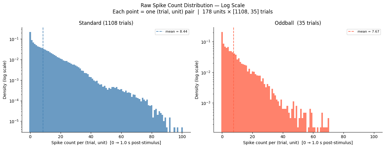
# Histogram of raw spike counts — log scale, standard and oddball on independent axes.
# For every (trial, unit) pair, count spikes in the post-stimulus window.
# Each data point is one unit on one trial — units, trials, and time are all preserved.
#
# The two axes are independent so each condition's density is judged on its own scale,
# making it easier to see distributional shape differences without one condition
# dominating the y-range.

def spike_counts_per_trial_unit(spike_times_list, stim_times, win_start, win_end):
    """Return (n_trials, n_units) integer array of spike counts in [win_start, win_end]
    relative to each stimulus onset."""
    n_t = len(stim_times)
    n_u = len(spike_times_list)
    out = np.zeros((n_t, n_u), dtype=np.int32)
    for u_i, u_spks in enumerate(spike_times_list):
        for t_i, t0 in enumerate(stim_times):
            i0, i1 = np.searchsorted(u_spks, [t0 + win_start, t0 + win_end])
            out[t_i, u_i] = i1 - i0
    return out


print("Computing raw spike counts (standard)...")
sc_std = spike_counts_per_trial_unit(spike_times_list, standard_times, 0.0, WINDOW_POST)
print(f"  shape: {sc_std.shape}  (trials × units)")

print("Computing raw spike counts (oddball)...")
sc_odd = spike_counts_per_trial_unit(spike_times_list, oddball_times, 0.0, WINDOW_POST)
print(f"  shape: {sc_odd.shape}  (trials × units)")

flat_std = sc_std.ravel()
flat_odd = sc_odd.ravel()

print(f"\nStandard: {len(flat_std):,} (trial, unit) pairs  |  mean = {flat_std.mean():.3f} spikes")
print(f"Oddball:  {len(flat_odd):,} (trial, unit) pairs  |  mean = {flat_odd.mean():.3f} spikes")

# Integer-aligned bins spanning both conditions
max_spk = max(flat_std.max(), flat_odd.max())
bins = np.arange(0, max_spk + 2) - 0.5

fig, axes = plt.subplots(1, 2, figsize=(13, 5))

for ax, flat, color, label in [
    (axes[0], flat_std, "steelblue", f"Standard ({len(standard_times)} trials)"),
    (axes[1], flat_odd, "tomato",    f"Oddball  ({len(oddball_times)} trials)"),
]:
    ax.hist(flat, bins=bins, density=True, color=color, alpha=0.8)
    ax.axvline(flat.mean(), color=color, lw=1.5, linestyle="--", alpha=0.9,
               label=f"mean = {flat.mean():.2f}")
    ax.set_yscale("log")
    ax.set_xlabel(f"Spike count per (trial, unit)  [0 → {WINDOW_POST} s post-stimulus]")
    ax.set_ylabel("Density (log scale)")
    ax.set_title(label)
    ax.legend(fontsize=8)
    ax.spines["top"].set_visible(False)
    ax.spines["right"].set_visible(False)

fig.suptitle(
    f"Raw Spike Count Distribution — Log Scale\n"
    f"Each point = one (trial, unit) pair  |  "
    f"{len(spike_times_list)} units × [{len(standard_times)}, {len(oddball_times)}] trials",
    fontsize=12,
)
plt.tight_layout()
plt.show()
Computing raw spike counts (standard)...
  shape: (1108, 178)  (trials × units)
Computing raw spike counts (oddball)...
  shape: (35, 178)  (trials × units)

Standard: 197,224 (trial, unit) pairs  |  mean = 8.441 spikes
Oddball:  6,230 (trial, unit) pairs  |  mean = 7.672 spikes
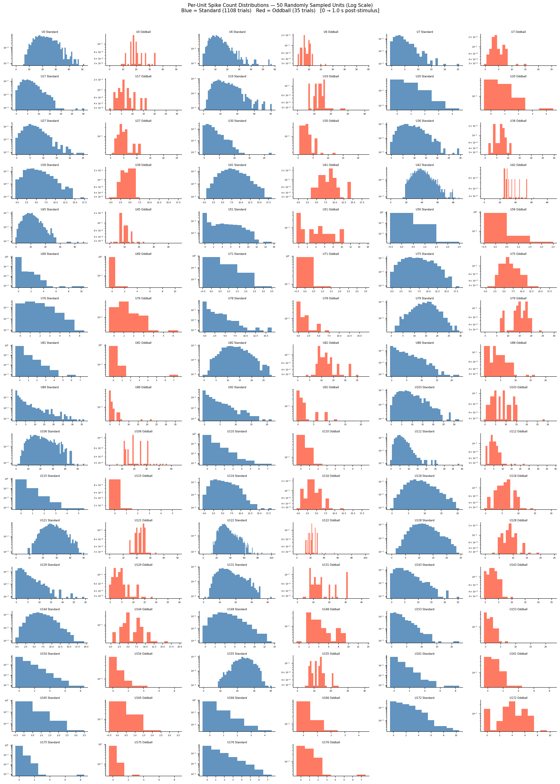
# Per-unit spike count distributions for 50 randomly sampled units
# Each unit occupies a Standard | Oddball pair of subplots (independent y-axes, log scale),
# mirroring the population plot above. Units are arranged 3 per row.

N_SAMPLE_UNITS   = 50
N_UNITS_PER_ROW  = 3
rng_samp = np.random.default_rng(seed=7)

n_avail = len(spike_times_list)
n_samp  = min(N_SAMPLE_UNITS, n_avail)
samp_idx = np.sort(rng_samp.choice(n_avail, size=n_samp, replace=False))
samp_spike_times = [spike_times_list[i] for i in samp_idx]

print(f"Sampled {n_samp} / {n_avail} units (seed=7).")

print("Computing spike counts for sampled units (standard)...")
sc_std_samp = spike_counts_per_trial_unit(samp_spike_times, standard_times, 0.0, WINDOW_POST)
print("Computing spike counts for sampled units (oddball)...")
sc_odd_samp = spike_counts_per_trial_unit(samp_spike_times, oddball_times,  0.0, WINDOW_POST)

# Grid: each unit = 2 adjacent columns (Standard left, Oddball right); N_UNITS_PER_ROW units per row
# figsize uses 3.0 w × 1.5 h per subplot → 2:1 width-to-height aspect ratio per panel
N_COLS = N_UNITS_PER_ROW * 2
N_ROWS = math.ceil(n_samp / N_UNITS_PER_ROW)

fig, axes = plt.subplots(N_ROWS, N_COLS, figsize=(3.0 * N_COLS, 1.5 * N_ROWS))

for u in range(n_samp):
    row      = u // N_UNITS_PER_ROW
    col_base = (u %  N_UNITS_PER_ROW) * 2
    ax_std   = axes[row, col_base]
    ax_odd   = axes[row, col_base + 1]

    counts_std_u = sc_std_samp[:, u]
    counts_odd_u = sc_odd_samp[:, u]

    max_spk_u = max(counts_std_u.max(), counts_odd_u.max(), 1)
    bins_u    = np.arange(0, max_spk_u + 2) - 0.5

    ax_std.hist(counts_std_u, bins=bins_u, density=True, color="steelblue", alpha=0.85)
    ax_odd.hist(counts_odd_u, bins=bins_u, density=True, color="tomato",    alpha=0.85)

    unit_label = f"U{samp_idx[u]}"
    ax_std.set_title(f"{unit_label} Standard",  fontsize=6, pad=2)
    ax_odd.set_title(f"{unit_label} Oddball",   fontsize=6, pad=2)

    for ax in (ax_std, ax_odd):
        ax.set_yscale("log")
        # which='both' ensures minor tick labels (2,3,4… between powers of 10 on log scale)
        # get the same size as major tick labels; without it they default to rcParams size.
        ax.tick_params(axis='both', which='both', labelsize=5)
        ax.spines["top"].set_visible(False)
        ax.spines["right"].set_visible(False)

# Hide any unfilled axes (if n_samp is not a multiple of N_UNITS_PER_ROW)
for j in range(n_samp * 2, N_ROWS * N_COLS):
    axes.ravel()[j].set_visible(False)

fig.suptitle(
    f"Per-Unit Spike Count Distributions — {n_samp} Randomly Sampled Units (Log Scale)\n"
    f"Blue = Standard ({len(standard_times)} trials)   "
    f"Red = Oddball ({len(oddball_times)} trials)   "
    f"[0 → {WINDOW_POST} s post-stimulus]",
    fontsize=11,
)
plt.tight_layout(rect=[0, 0, 1, 0.97])
plt.show()
Sampled 50 / 178 units (seed=7).
Computing spike counts for sampled units (standard)...
Computing spike counts for sampled units (oddball)...
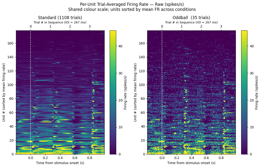
12. Firing Rate Heatmaps
Per-unit trial-averaged firing rates displayed as heatmaps, giving a compact view of which units respond to each stimulus condition and whether the response is enhanced or suppressed.
Two representations are shown:
Raw (spikes/s) — absolute firing rates on a shared colour scale so the standard and oddball conditions can be directly compared.
Z-scored, n-matched — standard trials are subsampled to match the oddball count before computing a pooled pre-stimulus baseline. Normalising this way removes the effect of trial-count asymmetry, and the difference panel (Oddball − Standard) highlights units with a genuine mismatch response.
# Raw (non-z-scored) trial-averaged firing rate heatmaps
# Shows absolute spike rates so the two conditions can be compared on the same physical scale
# before normalization.  Units sorted by mean firing rate (highest at top).
# fr_mean_std / fr_mean_odd: (n_units, n_bins) — computed above

mean_fr  = (fr_mean_odd.mean(axis=1) + fr_mean_std.mean(axis=1)) / 2  # pooled mean FR for sort
fr_sort  = np.argsort(mean_fr)[::-1]                                   # descending

# Shared colour range across both conditions
vmax_raw = np.nanpercentile(np.concatenate([fr_mean_std, fr_mean_odd]), 98)

fig, axes = plt.subplots(1, 2, figsize=(11, 7))

for ax, (data, title) in zip(axes, [
    (fr_mean_std[fr_sort], f"Standard ({len(standard_times)} trials)"),
    (fr_mean_odd[fr_sort], f"Oddball  ({len(oddball_times)} trials)"),
]):
    im = ax.imshow(data, aspect="auto",
                   extent=[window_t[0], window_t[-1], 0, data.shape[0]],
                   cmap="viridis", vmin=0, vmax=vmax_raw, origin="lower")
    ax.axvline(0, color="white", lw=1.2, linestyle="--", alpha=0.8)
    ax.set_xlabel("Time from stimulus onset (s)")
    ax.set_ylabel("Unit # (sorted by mean firing rate)")
    ax.set_title(title)
    plt.colorbar(im, ax=ax, label="Firing rate (spikes/s)")
    ax_top = ax.twiny()
    ax_top.set_xlim(window_t[0], window_t[-1])
    _n_back = int(np.floor(abs(window_t[0]) / ioi))
    _n_fwd  = int(np.floor(window_t[-1] / ioi))
    ax_top.set_xticks([n * ioi for n in range(-_n_back, _n_fwd + 1)
                       if window_t[0] <= n * ioi <= window_t[-1]])
    ax_top.set_xticklabels([str(n) for n in range(-_n_back, _n_fwd + 1)
                            if window_t[0] <= n * ioi <= window_t[-1]])
    ax_top.set_xlabel(f"Trial # in Sequence (IOI ≈ {ioi * 1000:.0f} ms)", fontsize=9)

fig.suptitle("Per-Unit Trial-Averaged Firing Rate — Raw (spikes/s)\n"
             "Shared colour scale; units sorted by mean FR across conditions",
             fontsize=12)
plt.tight_layout()
plt.show()
# Z-scored heatmap — n-matched standard trials
# standard_times has many more trials than oddball_times, which inflates the
# standard condition's pooled std and compresses the z-score scale.
# Here we randomly subsample standard trials (without replacement) to exactly
# match the oddball count, giving both conditions equal weight in the pooled
# normalisation and comparable trial-to-trial variability.

rng_match = np.random.default_rng(seed=42)
n_match   = len(oddball_times)
idx_sub   = rng_match.choice(len(standard_times), size=n_match, replace=False)
sampled_std_times = standard_times[idx_sub]

print(f"Subsampled standards: {len(sampled_std_times)} trials  "
      f"(matched to n_oddball={n_match};  original n_standard={len(standard_times)})")

print("Building trial-averaged spike rate (subsampled standard)...")
fr_mean_std_sub = get_trial_averaged_spike_rate(spike_times_list, sampled_std_times, bin_edges)

pre_mask = window_t < 0
eps      = 1e-6

baseline_mean_std_sub = fr_mean_std_sub[:, pre_mask].mean(axis=1, keepdims=True)
baseline_mean_odd_sub = fr_mean_odd[:, pre_mask].mean(axis=1, keepdims=True)

# Pooled pre-stimulus std uses both conditions at equal trial count
pooled_pre_sub  = np.concatenate(
    [fr_mean_std_sub[:, pre_mask], fr_mean_odd[:, pre_mask]], axis=1
)
pooled_norm_sub = pooled_pre_sub.std(axis=1, keepdims=True)

z_std_sub = (fr_mean_std_sub - baseline_mean_std_sub) / (pooled_norm_sub + eps)
z_odd_sub = (fr_mean_odd     - baseline_mean_odd_sub) / (pooled_norm_sub + eps)

cond_lim_sub = np.nanpercentile(np.abs(np.concatenate([z_std_sub, z_odd_sub])), 97)
diff_lim_sub = np.nanpercentile(np.abs(z_odd_sub - z_std_sub), 97)

datasets_sub = [
    (z_std_sub,               f"Standard — subsampled (n={n_match})", "RdBu_r", cond_lim_sub),
    (z_odd_sub,               f"Oddball (n={n_match})",               "RdBu_r", cond_lim_sub),
    (z_odd_sub - z_std_sub,   "Difference (Oddball − Standard)",      "RdBu_r", diff_lim_sub),
]

fig, axes = plt.subplots(1, 3, figsize=(16, 7),
                         gridspec_kw={"width_ratios": [1, 1, 1]})

for ax, (data, title, cmap, lim) in zip(axes, datasets_sub):
    clabel = "ΔZ-score" if "−" in title else "Z-score (baseline-normalised)"
    im = ax.imshow(data, aspect="auto",
                   extent=[window_t[0], window_t[-1], 0, data.shape[0]],
                   cmap=cmap, vmin=-lim, vmax=lim, origin="lower")
    ax.axvline(0, color="black", lw=1.2, linestyle="--", alpha=0.6)
    ax.set_xlabel("Time from stimulus onset (s)")
    ax.set_ylabel("Unit #")
    ax.set_title(title)
    plt.colorbar(im, ax=ax, label=clabel)
    ax_top = ax.twiny()
    ax_top.set_xlim(window_t[0], window_t[-1])
    _n_back = int(np.floor(abs(window_t[0]) / ioi))
    _n_fwd  = int(np.floor(window_t[-1] / ioi))
    ax_top.set_xticks([n * ioi for n in range(-_n_back, _n_fwd + 1)
                       if window_t[0] <= n * ioi <= window_t[-1]])
    ax_top.set_xticklabels([str(n) for n in range(-_n_back, _n_fwd + 1)
                            if window_t[0] <= n * ioi <= window_t[-1]])
    ax_top.set_xlabel(f"Trial # in Sequence (IOI ≈ {ioi * 1000:.0f} ms)", fontsize=9)

fig.suptitle(
    f"Per-Unit Stimulus-Aligned Firing Rate — n-matched comparison ({n_match} trials each)\n"
    "Z-scored: pooled temporal std from pre-stim baseline",
    fontsize=13)
plt.tight_layout()
plt.show()
Subsampled standards: 35 trials  (matched to n_oddball=35;  original n_standard=1108)
Building trial-averaged spike rate (subsampled standard)...
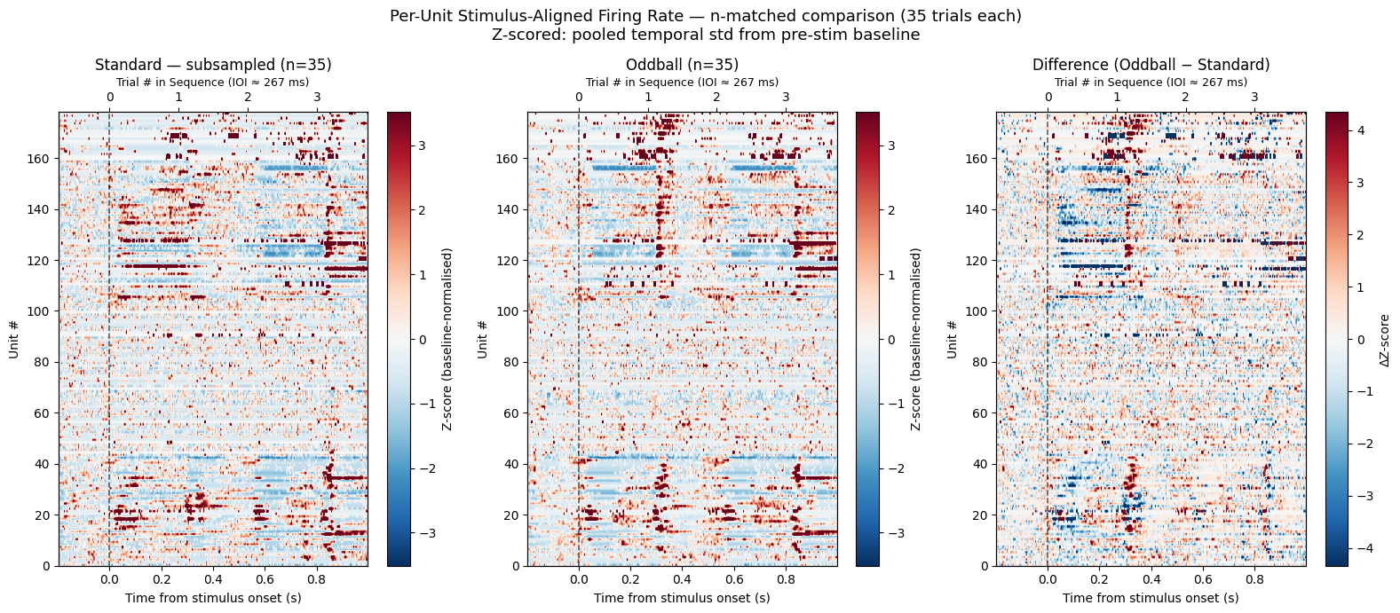
13. Stimulus-Aligned Average Response
We average across trials separately for oddball and standard presentations. Plotting both on the same axes reveals the mismatch response — the difference in activity between expected and unexpected stimuli. The three panels show:
Running speed — does the animal move differently after an oddball?
Pupil area — is there a general arousal response to the mismatch?
Population mean firing rate — for each trial, spikes from all quality units are binned and divided by the number of units to give a single population-average firing rate trace. Those per-trial traces are then averaged across trials to produce the plotted line.
Two helpers are defined inline:
get_stim_windows— slices fixed-length windows around each stimulus onset from an interpolated signal, yielding(n_trials, window_len)arrays for behavioral signals._plot_panel— computes mean ± SEM across trials for standard and oddball windows and draws both traces on one axis. To add or remove a panel, edit one entry in thepanelslist below.
Shaded regions show ±1 SEM across trials (i.e. trial-to-trial variability of the population-average firing rate; not variability across units).
# --- Helper: extract stimulus-aligned windows from an interpolated signal ---
def get_stim_windows(signal, stim_times, interp_hz, window_pre, window_post):
    """Extract fixed-length windows around each stimulus onset.
    Returns (n_trials, window_len) for 1-D signals."""
    wlen = int((window_post - window_pre) * interp_hz)
    n_t  = signal.shape[-1]
    slices = []
    for t in stim_times:
        i0 = int((t + window_pre) * interp_hz)
        i1 = i0 + wlen
        if 0 <= i0 and i1 <= n_t:
            slices.append(signal[..., i0:i1])
    if not slices:
        raise ValueError("No valid windows — check stim_times and window bounds.")
    return np.array(slices) if signal.ndim == 1 else np.stack(slices, axis=1)


# --- Helper: plot mean ± SEM for standard and oddball on one axis ---
def _plot_panel(ax, t, win_standard, win_oddball, show_legend=False):
    for wins, color, label in [
        (win_standard, "steelblue", f"Standard (n={len(standard_times)})"),
        (win_oddball,  "tomato",    f"Oddball  (n={len(oddball_times)})"),
    ]:
        n = wins.shape[0]
        m = np.nanmean(wins, axis=0)
        s = np.nanstd(wins, axis=0) / np.sqrt(n)
        ax.plot(t, m, color=color, lw=1.8, label=label)
        ax.fill_between(t, m - s, m + s, color=color, alpha=0.25)
    ax.axvline(0, color="black", lw=1.0, linestyle="--")
    if show_legend:
        ax.legend(fontsize=8)
    ax.spines["top"].set_visible(False)
    ax.spines["right"].set_visible(False)


# --- Extract behavioral windows ---
window_t_behav = np.linspace(WINDOW_PRE, WINDOW_POST,
                              int((WINDOW_POST - WINDOW_PRE) * INTERP_HZ))

run_win_std = get_stim_windows(interp_running, standard_times, INTERP_HZ, WINDOW_PRE, WINDOW_POST)
run_win_odd = get_stim_windows(interp_running, oddball_times,  INTERP_HZ, WINDOW_PRE, WINDOW_POST)
eye_win_std = get_stim_windows(interp_eye, standard_times, INTERP_HZ, WINDOW_PRE, WINDOW_POST)
eye_win_odd = get_stim_windows(interp_eye, oddball_times,  INTERP_HZ, WINDOW_PRE, WINDOW_POST)

print(f"Behavioral windows — oddball: {run_win_odd.shape},  standard: {run_win_std.shape}")

# --- Plot: 3 panels sharing the same x-axis ---
# To add or remove a panel, add/remove one tuple from this list.
fig, axes = plt.subplots(3, 1, figsize=(10, 11), sharex=True,
                          gridspec_kw={"height_ratios": [1, 1, 1.6]})

panels = [
    (axes[0], window_t_behav, run_win_std,       run_win_odd,
     "Running speed",         "Running Speed"),
    (axes[1], window_t_behav, eye_win_std,        eye_win_odd,
     "Pupil area (pixels²)",  "Eye Tracking (Pupil Area)"),
    (axes[2], window_t,       fr_per_trial_std,   fr_per_trial_odd,
     "Mean firing rate\n(spikes/s)",
     f"Population Mean Firing Rate\n"
     f"({len(spike_times_list)} units avg'd per trial; ±1 SEM across trials)"),
]

for i, (ax, t, win_std, win_odd, ylabel, title) in enumerate(panels):
    _plot_panel(ax, t, win_std, win_odd, show_legend=(i == 0))
    ax.set_ylabel(ylabel)
    ax.set_title(title)

axes[0].set_xlim(window_t_behav[0], window_t_behav[-1])
axes[2].set_xlabel("Time from stimulus onset (s)")

# Secondary x-axis on the top panel showing trial numbers in sequence
ax_top = axes[0].twiny()
ax_top.set_xlim(window_t_behav[0], window_t_behav[-1])
_n_back = int(np.floor(abs(window_t_behav[0]) / ioi))
_n_fwd  = int(np.floor(window_t_behav[-1] / ioi))
ax_top.set_xticks([n * ioi for n in range(-_n_back, _n_fwd + 1)
                   if window_t_behav[0] <= n * ioi <= window_t_behav[-1]])
ax_top.set_xticklabels([str(n) for n in range(-_n_back, _n_fwd + 1)
                        if window_t_behav[0] <= n * ioi <= window_t_behav[-1]])
ax_top.set_xlabel(f"Trial # in Sequence (IOI ≈ {ioi * 1000:.0f} ms)", fontsize=9)

fig.suptitle("Stimulus-Aligned Average Response\nOddball vs. Standard (±1 SEM across trials)",
             fontsize=13)
plt.tight_layout()
plt.show()
Behavioral windows — oddball: (35, 120), standard: (1108, 120)
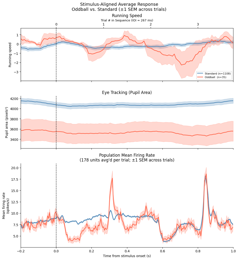
14. Summary
This notebook demonstrated how to access and visualize the key data streams in a Predictive Processing Neuropixels NWB file:
| Data type | NWB location | Key attributes |
|---|---|---|
| Probe devices | nwb.devices | probe name, model, description |
| Electrode table | nwb.electrodes | group_name, location, x/y/z |
| Units | nwb.units | spike_times, snr, firing_rate, waveform_mean |
| Running wheel (raw) | nwb.acquisition["raw_running_wheel_rotation"] | .data, .timestamps |
| Eye tracking | nwb.processing['eye_tracking']['pupil'] | .area, .timestamps |
| LFP | nwb.processing['ecephys']['LFP'].electrical_series[key] | .data (time × ch), .timestamps |
| Stimulus tables | nwb.intervals[name] | start_time, stop_time, TrialType |
Community Resources
GitHub Discussions — for questions, ideas, and collaboration
- Zhou, Z., Huang, W. A., Yu, Y., Negahbani, E., Stitt, I. M., Alexander, M., Hamm, J. P., Kato, H. K., & Fröhlich, F. (2020). Stimulus-specific regulation of visual oddball differentiation in posterior parietal cortex. Scientific Reports, 10, 13973. 10.1038/s41598-020-70448-6
- Hamm, J. P., Shymkiv, Y., Han, S., Yang, W., & Yuste, R. (2021). Cortical ensembles selective for context. Proceedings of the National Academy of Sciences, 118. 10.1073/pnas.2026179118
- Pak, A., Kissinger, S. T., & Chubykin, A. A. (2021). Impaired adaptation and laminar processing of the oddball paradigm in the primary visual cortex of Fmr1 KO mouse. Frontiers in Cellular Neuroscience, 15, 668230. 10.3389/fncel.2021.668230
- Homann, J., Koay, S. A., Chen, K. S., Tank, D. W., & II, M. J. B. (2022). Novel stimuli evoke excess activity in the mouse primary visual cortex. Proceedings of the National Academy of Sciences, 119. 10.1073/pnas.2108882119
- Jordan, R., & Keller, G. B. (2020). Opposing influence of top-down and bottom-up input on excitatory layer 2/3 neurons in mouse primary visual cortex. Neuron, 108, 1194-1206.e5. 10.1016/j.neuron.2020.09.024
- Huang, Y., Shamsnia, A., Chen, M., Wu, S., Stamm, T., Medico, S., & Najafi, F. (2025). Intrinsic timing, not temporal prediction, underlies ramping dynamics in visual and parietal cortex during passive behavior. bioRxiv. 10.1101/2025.09.11.673960