Marker panel generation • mfishtools

This vignette demonstrates how to generate an optimal marker gene panel (of length N), and then predicts how well each of the FACs cells map into the types defined as a measure of panel quality.

The strategy used is a correlation-baseed greedy algorithm, which aims to minimize the distance between the actual and predicted clusters (rather than maximizing the fraction correctly mapping to each cluster).

Workspace set-up

Install the necessary packages. In this case we are using data from tasic2016data and plotting functions from scrattch.vis.

install.packages("devtools")
devtools::install_github("AllenInstitute/scrattch.vis")  # For plotting
devtools::install_github("AllenInstitute/tasic2016data") # For our data example

Load libraries.

suppressPackageStartupMessages({
  library(mfishtools)    # This library!
  library(gplots)        # This is for plotting gene panels only.
  library(scrattch.vis)  # This is for plotting gene panels only.
  library(matrixStats)   # For rowMedians function, which is fast
  library(tasic2016data) # For the data
})
options(stringsAsFactors = FALSE)  # IMPORTANT
print("Libraries loaded.")

## [1] "Libraries loaded."

Read in the data (in this case we will use the Tasic 2016 data, which includes ~1800 cells from mouse primary visual cortex).

annotations <- tasic_2016_anno
counts      <- tasic_2016_counts
rpkm        <- tasic_2016_rpkm
annotations <- annotations[match(colnames(counts),annotations$sample_name),]  # Put them in the correct order

Data preparations

This analysis will only be looking at marker genes for GABAergic neurons, so we need to only consider cells mapping to GABAergic types. We also define some convenient cluster info variables here.

clusterType = annotations$broad_type 
includeClas = "GABA-ergic Neuron"  # In this analysis, we are only considering interneurons
excludeClas = sort(setdiff(clusterType,includeClas))
gliaClas    = setdiff(excludeClas,"Glutamatergic Neuron") 
kpSamp      = !is.element(clusterType,excludeClas)
anno        = annotations[kpSamp,]
cl          = annotations$primary_type_label
names(cl)   = annotations$sample_name
kpClust     = sort(unique(cl[kpSamp]))
gliaClust   = sort(unique(cl[is.element(clusterType,gliaClas)]))

Convert the data to log2(rpkm). NOTE: we often use counts per million of introns + exons when performing this analysis. Currently, we don’t know which method produces more reliable markers. Alternative code for calculating cpm is commented out below.

normDat = log2(rpkm+1)
#sf      = colSums(counts)/10^6
#cpms    = t(t(counts)/sf)
#normDat = log2(cpms+1)

Calculate proportions and medians. These are both needed for gene filtering and for marker selection.

exprThresh = 1
medianExpr = do.call("cbind", tapply(names(cl), cl, function(x) rowMedians(normDat[,x]))) 
propExpr   = do.call("cbind", tapply(names(cl), cl, function(x) rowMeans(normDat[,x]>exprThresh))) 
rownames(medianExpr) <- rownames(propExpr) <- genes <- rownames(normDat)

Combinatorial marker gene selection

This section is where gene selection happens. There are two steps: (1) gene filtering and (2) marker selection, both of which are described below.

We first want to define some gene filters prior to running gene selection. Note that this filtering occurs prior to gene selection and does not occur during the selection process. To see details about all of the specific filters, see the code block below or use ?filterPanelGenes. Overall, the goal of this section is to exclude genes that won’t work properly with the specific spatial transcriptomics method desired because their expression is too low or too high, or they are too short. It also removes genes with too much off-target expression, genes that are expressed in too many cell types, and genes that are potentially not of interest because they are unannotated, or on a sex chromosome, or are don’t work for any other reason. It also takes the most binary genes as the possible selection space in order to try and avoid genes whose only cell type differences are in magnitude. In this case, we will use a total of 250 binary genes.

startingGenePanel <-  c("Gad1","Slc32a1","Pvalb","Sst","Vip")
runGenes <- NULL
runGenes <- filterPanelGenes(
  summaryExpr = 2^medianExpr-1,  # medians (could also try means); We enter linear values to match the linear limits below
  propExpr    = propExpr,    # proportions
  onClusters  = kpClust,     # clusters of interest for gene panel
  offClusters = gliaClust,   # clusters to exclude expression
  geneLengths = NULL,        # vector of gene lengths (not included here)
  startingGenes  = startingGenePanel,  # Starting genes (from above)
  numBinaryGenes = 250,      # Number of binary genes (explained below)
  minOn     = 10,   # Minimum required expression in highest expressing cell type
  maxOn     = 500,  # Maximum allowed expression
  maxOff    = 50,   # Maximum allowed expression in off types (e.g., aviod glial expression)
  minLength = 960,  # Minimum gene length (to allow probe design; ignored in this case)
  fractionOnClusters = 0.5,  # Max fraction of on clusters (described above)
  excludeGenes    = NULL,    # Genes to exclude.  Often sex chromosome or mitochondrial genes would be input here.
  excludeFamilies = c("LOC","Fam","RIK","RPS","RPL","\\-","Gm","Rnf","BC0")) # Avoid LOC markers, in this case

## 1278 total genes pass constraints prior to binary score calculation.

The second step is our marker panel selection. This strategy uses a greedy algorithm to iteratively add the “best” gene to the existing panel until the panel reaches a certain size. Specifically, each cell in the reference data set is correlated with each cluster median using the existing marker gene set, and the most highly correlated cluster is compared with the originally assigned cluster for each cell. By default the algorithm tries to optimize the fraction of cells correctly mapping to each cluster by using this correlation-based mapping. An alternative strategy that is particularly useful for smaller gene panels is to use a weighting strategy to penalize cells that map to a distant cluster more than cells that map to a nearby cluster. To do this we iteratively choose genes from the starting gene panel such that the addition of each gene minimizes the correlation distance between clusters.

To do this we first determine the cluster distance based on correlation of top binary genes, which is what is done in this code block.

corDist         <- function(x) return(as.dist(1-cor(x)))
clusterDistance <- as.matrix(corDist(medianExpr[runGenes,kpClust]))
print(dim(clusterDistance))

## [1] 23 23

This step constructs the gene panel, as described above. Once again, use ?buildMappingBasedMarkerPanel and see the code block below for details on the parameters, but there are a few key options. First, we find it useful to subsample cells from each cluster which decreases the time for the algorithm to run and also more evenly weights the clusters for gene selection.

fishPanel <- buildMappingBasedMarkerPanel(
  mapDat        = normDat[runGenes,kpSamp],     # Data for optimization
  medianDat     = medianExpr[runGenes,kpClust], # Median expression levels of relevant genes in relevant clusters
  clustersF     = cl[kpSamp],                   # Vector of cluster assignments
  panelSize     = 30,                           # Final panel size
  currentPanel  = startingGenePanel,            # Starting gene panel
  subSamp       = 15,                           # Maximum number of cells per cluster to include in analysis (20-50 is usually best)
  optimize      = "CorrelationDistance",        # CorrelationDistance maximizes the cluster distance as described
  clusterDistance = clusterDistance,            # Cluster distance matrix
  percentSubset = 50                            # Only consider a certain percent of genes each iteration to speed up calculations (in most cases this is not recommeded)
)

##

## [1] "Added Necab1 with average cluster distance 0.248 [ 5 ]."
## [1] "Added Col25a1 with average cluster distance 0.212 [ 6 ]."
## [1] "Added Thsd7a with average cluster distance 0.184 [ 7 ]."
## [1] "Added Adarb2 with average cluster distance 0.166 [ 8 ]."
## [1] "Added Adra1b with average cluster distance 0.15 [ 9 ]."
## [1] "Added Crh with average cluster distance 0.138 [ 10 ]."
## [1] "Added Sstr1 with average cluster distance 0.126 [ 11 ]."
## [1] "Added Trp53i11 with average cluster distance 0.121 [ 12 ]."
## [1] "Added Cpne2 with average cluster distance 0.111 [ 13 ]."
## [1] "Added Rgs12 with average cluster distance 0.104 [ 14 ]."
## [1] "Added Npy2r with average cluster distance 0.0989 [ 15 ]."
## [1] "Added Cbln4 with average cluster distance 0.0926 [ 16 ]."
## [1] "Added Grpr with average cluster distance 0.0907 [ 17 ]."
## [1] "Added Crispld2 with average cluster distance 0.0874 [ 18 ]."
## [1] "Added Cacna2d1 with average cluster distance 0.0826 [ 19 ]."
## [1] "Added Cplx3 with average cluster distance 0.078 [ 20 ]."
## [1] "Added Sorcs1 with average cluster distance 0.0746 [ 21 ]."
## [1] "Added Npas1 with average cluster distance 0.0705 [ 22 ]."
## [1] "Added Tacstd2 with average cluster distance 0.0694 [ 23 ]."
## [1] "Added Ttc39b with average cluster distance 0.0678 [ 24 ]."
## [1] "Added Gpc3 with average cluster distance 0.0675 [ 25 ]."
## [1] "Added Nek7 with average cluster distance 0.066 [ 26 ]."
## [1] "Added Cacna1e with average cluster distance 0.0629 [ 27 ]."
## [1] "Added Olfm3 with average cluster distance 0.0604 [ 28 ]."
## [1] "Added Ano3 with average cluster distance 0.0576 [ 29 ]."

This is the panel!

Assess panel quality

First, let’s plot the panel in the context of the clusters we care about. This can be done using the scrattch.vis library.

plotGenes <- fishPanel
plotData  <- cbind(sample_name = colnames(rpkm), as.data.frame(t(rpkm[plotGenes,])))
clid_inh  <- 1:23  # Cluster IDs for inhibitory clusters

# violin plot example.  Could be swapped with fire, dot, bar, box plot, heatmap, Quasirandom, etc.
sample_fire_plot(data = plotData, anno = annotations, genes = plotGenes, grouping = "primary_type", 
                 log_scale=TRUE, max_width=15, label_height = 8, group_order = clid_inh)

The first half of this panel looks like most of the genes have fairly distinct and binarized patterning, while many of the genes in the latter half of the panel appear to be showing redundant information, suggesting that after a certain point this strategy becomes less than optimal in a practical sense.

How do they look across ALL cell types (realizing that we don’t expect to see all these types in the tissue we care about)?

sample_fire_plot(data = plotData, anno = annotations, genes = plotGenes, grouping = "primary_type", 
                 log_scale=TRUE, max_width=15, label_height = 8)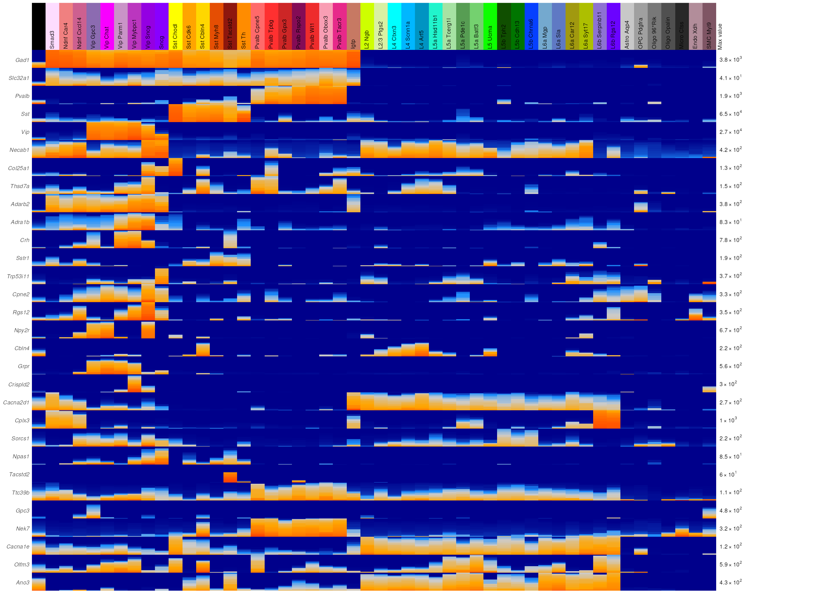

We get a little bit of excitatory and glial cell separation for free, but it’s not great (as expected).

What fraction of cells are correctly mapped to leaf nodes? Note that we don’t necessarily expect this number to be high. Also note that this is using all of the above genes, so will actually be higher than we would get with any given 9-gene panel.

assignedCluster <- suppressWarnings(getTopMatch(corTreeMapping(mapDat = normDat[runGenes,kpSamp], 
                   medianDat=medianExpr[runGenes,kpClust], genesToMap=fishPanel)))
print(paste0("Percent correctly mapped: ",signif(100*mean(as.character(assignedCluster$TopLeaf)==cl[kpSamp],na.rm=TRUE),3),"%"))

## [1] "Percent correctly mapped: 68.5%"

Around ~72% of the cells are correctly mapped with this panel, which is reasonable, but less than ideal. How does the plot look for fewer genes?

fractionCorrectWithGenes(fishPanel,normDat[,kpSamp],medianExpr[runGenes,kpClust],cl[kpSamp],
                         main="Mapping quality for different numbers of included genes",return=FALSE)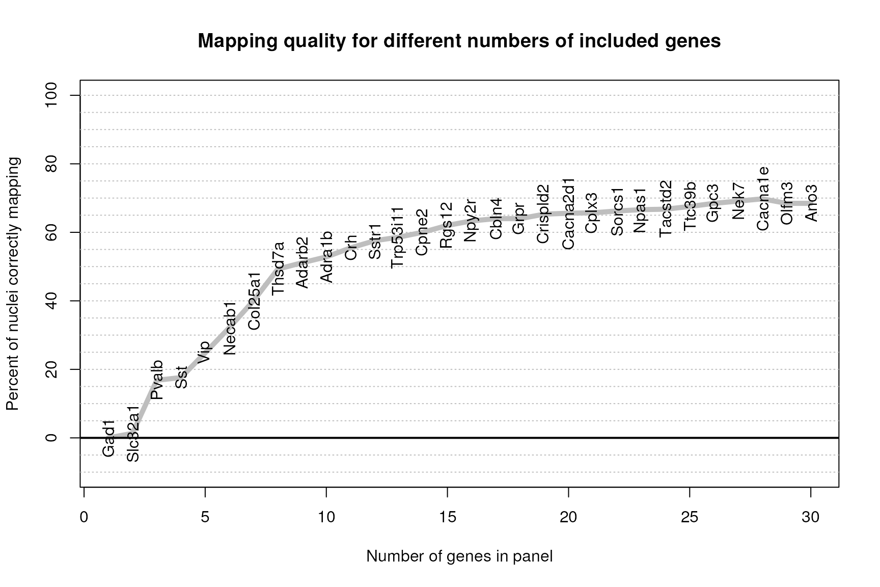

This plot suggests that with 30 genes we are continuing to see improvement by adding new genes; however, by approximately a 20 gene panel the level of improvement decreases dramatically for each gene added. Later releases of this library will include additional strategies for optimizing the panel beyond these initial 20 or so genes.

Finally, as an overview, we create a confusion matrix based on the top leaf assignments. This will let us address which pairs of clusters are the most confused. Are they adjacent/nearby on the tree? Note that the colors are distorted to highlight confusion in the tree.

membConfusionProp  <- getConfusionMatrix(cl[kpSamp],assignedCluster[,1],TRUE)
clOrd <- (annotations$primary_type_label[match(clid_inh,annotations$primary_type_id)])  # Cluster order
heatmap.2(pmin(membConfusionProp,0.25)[clOrd,clOrd],Rowv=FALSE,Colv=FALSE,trace="none",dendrogram="none",
          margins=c(16,16),main="Confusion Matrix")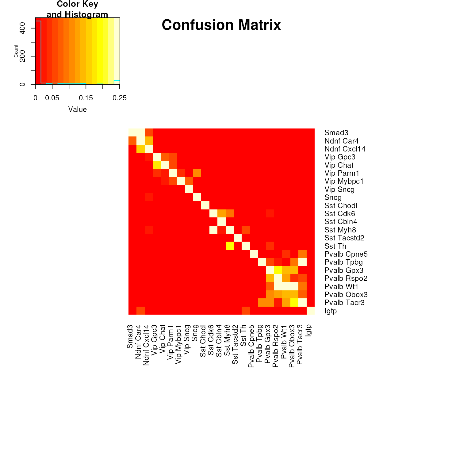

Most of the errors are nearby on the diagonal, which is what we were optimizing for using the clusterDistance strategy.