
Working with annotation volumes#
Annotation volumes are useful references for understanding brain parcellations at multiple levels. For example, a cell’s location can be described as being in the lateral geniculate nucleus or in any of its parent structures in the anatomical ontology (dorsal thalamus, thalamus, diencephalon, etc.). Annotation volumes can label CCF-registered data with terms from the HOMBA ontology.
This tutorial shows some examples for using the human HOMBA annotation volume to (1) query labels and (2) extract regions at any level as a mask for reference and visualization.
import pandas as pd
from pathlib import Path
from atlas_utils.annotation import Annotation
First, we will read in the annotation volume from the local directory. In this tutorial, we will assume that you have already downloaded the annotation volumes using the download_atlas method (see Getting started).
The annotation image is an array where each voxel is assigned a numeric annotation value that corresponds to the most granular structure that is annotated in the volume. To convert the numeric value to a label, we will need to import the terminology.csv table.
directory = "./data/atlases/hmba-adult-human-homba-atlas/2025/" #Change to local path if data is downloaded elsewhere

dir_path = Path(directory)
image_filepath = dir_path / "annotations_compressed_700.nii.gz"
terminology_filepath = dir_path / "terminology.csv"
annotation_image = Annotation.from_file(image_filepath, terminology_filepath)

print(f"Annotation image has dimensions: {annotation_image.npy.shape}")
Annotation image has dimensions: (260, 311, 260)
The terminology table contains the annotation label value as well as the label name, acronym, and associated metadata (eg. color).
annotation_image.terminology.head(10)
| identifier | annotation_value | parent_identifier | name | abbreviation | color_hex_triplet | descendant_identifiers | descendants | descendant_annotation_values | |
|---|---|---|---|---|---|---|---|---|---|
| 0 | HOMBA:10154 | 501 | NaN | central nervous system (neural tube) | CNS | #3cb44b | ['HOMBA:10154', 'HOMBA:10155', 'HOMBA:AA30000'... | ['HOMBA:10154', 'HOMBA:10155', 'HOMBA:AA30000'... | [501, 502, 503, 84, 504, 505, 506, 507, 508, 5... |
| 1 | HOMBA:10155 | 502 | HOMBA:10154 | brain | Br | #808000 | ['HOMBA:10155', 'HOMBA:AA30000', 'HOMBA:10156'... | ['HOMBA:10155', 'HOMBA:AA30000', 'HOMBA:10156'... | [502, 503, 84, 504, 505, 506, 507, 508, 509, 5... |
| 2 | HOMBA:AA30000 | 503 | HOMBA:10155 | gray matter of brain | BGM | #0082c8 | ['HOMBA:AA30000', 'HOMBA:10156', 'HOMBA:10158'... | ['HOMBA:AA30000', 'HOMBA:10156', 'HOMBA:10158'... | [503, 84, 504, 505, 506, 507, 508, 509, 510, 5... |
| 3 | HOMBA:10156 | 84 | HOMBA:AA30000 | gray matter of forebrain (prosencephalon) | FB | #000080 | ['HOMBA:10156', 'HOMBA:10158', 'HOMBA:10159', ... | ['HOMBA:10156', 'HOMBA:10158', 'HOMBA:10159', ... | [84, 504, 505, 506, 507, 508, 509, 510, 511, 5... |
| 4 | HOMBA:10158 | 504 | HOMBA:10156 | telencephalon | Tel | #e6194b | ['HOMBA:10158', 'HOMBA:10159', 'HOMBA:10160', ... | ['HOMBA:10158', 'HOMBA:10159', 'HOMBA:10160', ... | [504, 505, 506, 507, 508, 509, 510, 511, 512, ... |
| 5 | HOMBA:10159 | 505 | HOMBA:10158 | cerebral cortex | Cx | #000080 | ['HOMBA:10159', 'HOMBA:10160', 'HOMBA:AA30001'... | ['HOMBA:10159', 'HOMBA:10160', 'HOMBA:AA30001'... | [505, 506, 507, 508, 509, 510, 511, 512, 513, ... |
| 6 | HOMBA:10160 | 506 | HOMBA:10159 | neocortex (isocortex) | NCx | #ffd7b4 | ['HOMBA:10160', 'HOMBA:AA30001', 'HOMBA:10161'... | ['HOMBA:10160', 'HOMBA:AA30001', 'HOMBA:10161'... | [506, 507, 508, 509, 510, 511, 512, 513, 514, ... |
| 7 | HOMBA:AA30001 | 507 | HOMBA:10160 | regions (areas) of neocortex | NCxR | #000080 | ['HOMBA:AA30001', 'HOMBA:10161', 'HOMBA:10172'... | ['HOMBA:AA30001', 'HOMBA:10161', 'HOMBA:10172'... | [507, 508, 509, 510, 511, 512, 513, 514, 515, ... |
| 8 | HOMBA:10161 | 508 | HOMBA:AA30001 | frontal cortex | FCx | #008080 | ['HOMBA:10161', 'HOMBA:10172', 'HOMBA:10190', ... | ['HOMBA:10161', 'HOMBA:10172', 'HOMBA:10190', ... | [508, 509, 510, 511, 512, 513, 514, 515, 516, ... |
| 9 | HOMBA:10172 | 509 | HOMBA:10161 | prefrontal cortex | PFC | #f032e6 | ['HOMBA:10172', 'HOMBA:10190', 'HOMBA:10191', ... | ['HOMBA:10172', 'HOMBA:10190', 'HOMBA:10191', ... | [509, 510, 511, 512, 513, 514, 515, 516, 517, ... |
1. Query annotation labels from coordinates#
Now that we have loaded in the annotation and terminology, we can use these data assets to query (x,y,z) coordinates and get the anatomical structure label for that coordinate voxel. Coordinates can be represented either by the array index or the physical space. Physical space coordinates refer to the anterior commissure as the origin and represent distances in mm from the origin in (x,y,z)
Let’s use the physical point [17.1, 0.7, -0.6] as a reference
query_coordinate = [17.1, 0.7, -0.6]
acronym, name = annotation_image.get_atlas_label(query_coordinate, physical_coordinate = True)

print(f"Coordinate {query_coordinate} is in {acronym}: {name}")
Coordinate [17.1, 0.7, -0.6] is in GPe: external division of globus pallidus
Note: physical coordinates from the neuroglancer visualization have a correction factor, which is applied by setting neuroglancer_coordinate=True.
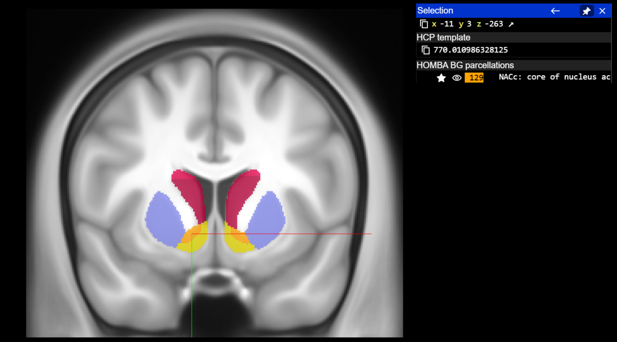
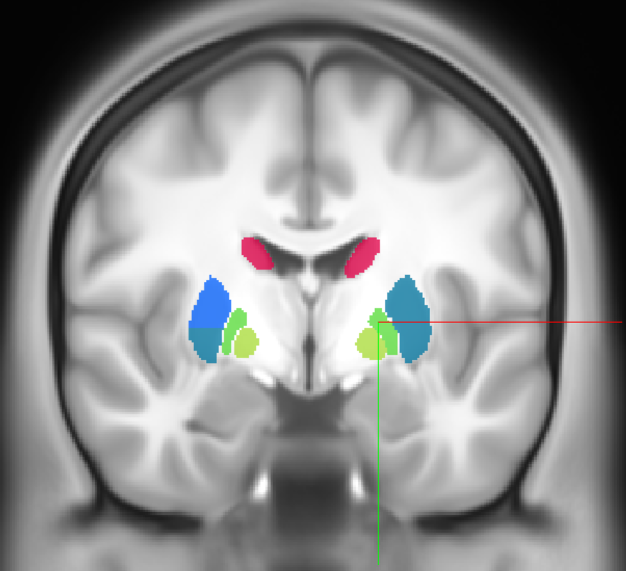
query_coordinate_neuroglancer = [-11, 3, -263]
acronym, name = annotation_image.get_atlas_label(query_coordinate_neuroglancer, physical_coordinate = True, neuroglancer_coordinate=True)

print(f"Coordinate {query_coordinate_neuroglancer} is in {acronym}: {name}")
Coordinate [-11, 3, -263] is in NACc: core of nucleus accumbens
1.1 Assign annotation labels to existing data table#
Often, we will have sets of coordinates that define points/landmarks of interest (eg. soma locations). Rather than labeling them individually, we can annotate the input data table with the appropriate anatomical labels.
Here, we will use a short example of randomly sampled points throughout the basal ganglia. In this example, the coordinates are indices rather than in physical dimensions (note that physical_coordinate=False)
input_data_filename = "./data/example_coordinates.csv"
input_data = pd.read_csv(input_data_filename)
input_data.head(5)
| identifier | x | y | z | |
|---|---|---|---|---|
| 0 | cell01 | 148 | 191 | 131 |
| 1 | cell02 | 155 | 189 | 87 |
| 2 | cell03 | 158 | 139 | 131 |
| 3 | cell04 | 107 | 177 | 108 |
| 4 | cell05 | 86 | 167 | 89 |
labeled_data = annotation_image.label_csv(input_data, physical_coordinate=False)
labeled_data.head(5)
| identifier | x | y | z | abbreviation | name | |
|---|---|---|---|---|---|---|
| 0 | cell01 | 148 | 191 | 131 | CaB | body of caudate nucleus |
| 1 | cell02 | 155 | 189 | 87 | PuR | rostral putamen |
| 2 | cell03 | 158 | 139 | 131 | CaT | tail of caudate nucleus (caudolateral division... |
| 3 | cell04 | 107 | 177 | 108 | GPe | external division of globus pallidus |
| 4 | cell05 | 86 | 167 | 89 | PuCv | ventral subdivision of PuC |
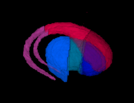
2. Create region masks#
Annotation volumes can also be used to generate region masks for visualization or as a reference. For example, we may need to create a volume for the dorsal striatum for downstream use in visualizing region boundaries. However, the annotation volumes only show the most granular structures. To create a volume for the dorsal striatum, we will need to combine and aggregate all structures that are part of the dorsal striatum.
This can be done using the Annotation object we created earlier and the structure acronym
save_filename = dir_path / "dorsal_striatum_mask.nii.gz" # Or wherever you'd like to save it
annotation_image.create_region_mask('DS', save_filename)
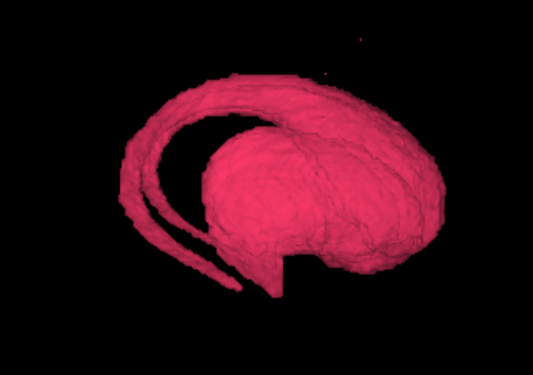
This creates a volume that can be used for masking and visualization. We can also use this mask to create a new annotation from file for querying for region identity.
2.1 Get descendant structure names#
Related to the above example, we may need to get a list of descendant structures associated with a region, eg. which labeled structures are part of dorsal striatum?
The annotation.terminology dataframe contains descendant identifiers and label values. However, to convert the identfiers into full names and acroynms, we can use the annotation object to query a structure and return its descendants.
query_structure = 'DS'
descendant_acronym, descendant_name = annotation_image.get_descendants(query_structure)
print(f"Descendants of {query_structure}: {descendant_acronym}")
print(f"Descendants of {query_structure}: {descendant_name}")
Descendants of DS: ['DS', 'Ca', 'CaH', 'CaHld', 'CaHmv', 'CaB', 'CaBld', 'CaBmv', 'CaT', 'CaTd', 'CaTv', 'Eca', 'Pu', 'PuR', 'PuRld', 'PuRmv', 'PuM', 'PuMld', 'PuMmv', 'IPAC', 'IPACm', 'IPACl', 'PuC', 'PuCld', 'PuCmv', 'PuCv', 'AStr', 'PuMG', 'CaPu']
Descendants of DS: ['dorsal striatum (caudoputamen complex-CP, STRd)', 'caudate nucleus (mediodorsal division of the CP)', 'head of caudate nucleus', 'laterodorsal subdivision of CaH', 'medioventral subdivision of CaH', 'body of caudate nucleus', 'laterodorsal subdivision of CaB', 'medioventral subdivision of CaB', 'tail of caudate nucleus (caudolateral division of the CP)', 'dorsal subdivision of CaT', 'ventral subdivision of CaT', 'peri-caudate ependymal and subependymal zone', 'putamen (lateroventral division of the CP)', 'rostral putamen', 'laterodorsal subdivision of PuR', 'medioventral subdivision of PuR', 'middle putamen', 'laterodorsal subdivision of PuM', 'medioventral subdivision of PuM', 'interstitial nucleus of posterior limb of anterior commissure (fundus of striatum)', 'medial part of IPAC', 'Lateral part of IPAC', 'caudal putamen', 'laterodorsal subdivision of PuC', 'medioventral subdivision of PuC', 'ventral subdivision of PuC', 'amygdalostriatal transition area', 'marginal division (cell groups) of putamen', 'caudate-putamen cell bridges']