OpenScope’s Texture Dataset - OpenScope Databook

How do mice internally represent complex visual stimuli, and how do they use this information to guide behavior during decision making? In this project, we focused on visual textures: images composed of repeated patterns that obey translational, rotational, or scale symmetries. These textures are common in the natural world and provide important cues for identifying objects and their properties.

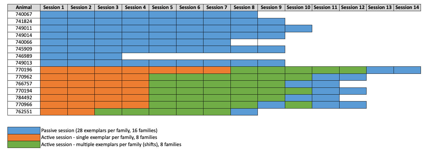
The Texture Dataset consists of 2 animal cohorts. A naive one, in which mice were shown the same set of visual textures across multiple sessions (16 different textures families, with 28 images per family, also called exemplars). And a trained one, in which mice were first trained in a visually-guided discrimination task involving textures. Mice were initially trained following the standard change-detect Visual Behavior optical Physiology protocol. After the training stage with gratings was completed, mice were switched toa a new task involving the texture images instead. This task (orange) mimicked the original “familiar images” task protocol, but instead used a new set of texture images (8 families, 1 exemplar per family). So 8 different images in total. After learning this stage, ,mice were switched to the final task (in green) where they had to visually discriminate between image families (rather than just images). To that end, what would typically be a set of consecutive trials with the same image (no-go trials) was replaced by a set of different images from the same family (exemplars). That is, mice had to visually discriminate between texture families (e.g., images of rocks vs images of leaves), rather than just different stimulii. After 4-5 sessions in this task, the mice were switched to the same passive viewing protocol (blue) as the naive mice.

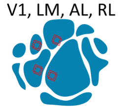
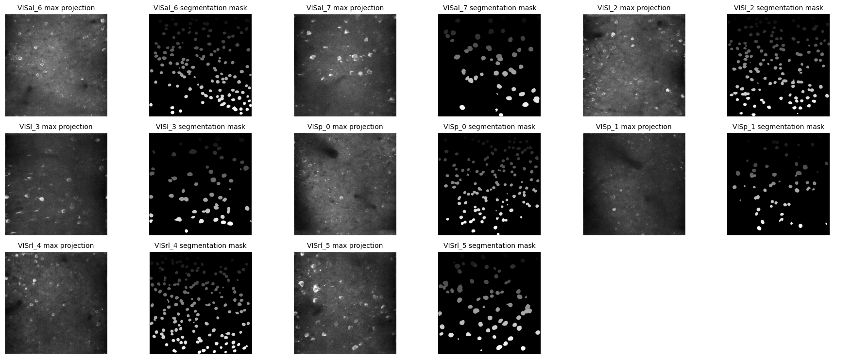
Imaging consisted of multi-plane imaging across 4 areas (V1, LM, AL, RL) and 2 depths (layers 2/3 and 5).

All texture families used (passive session):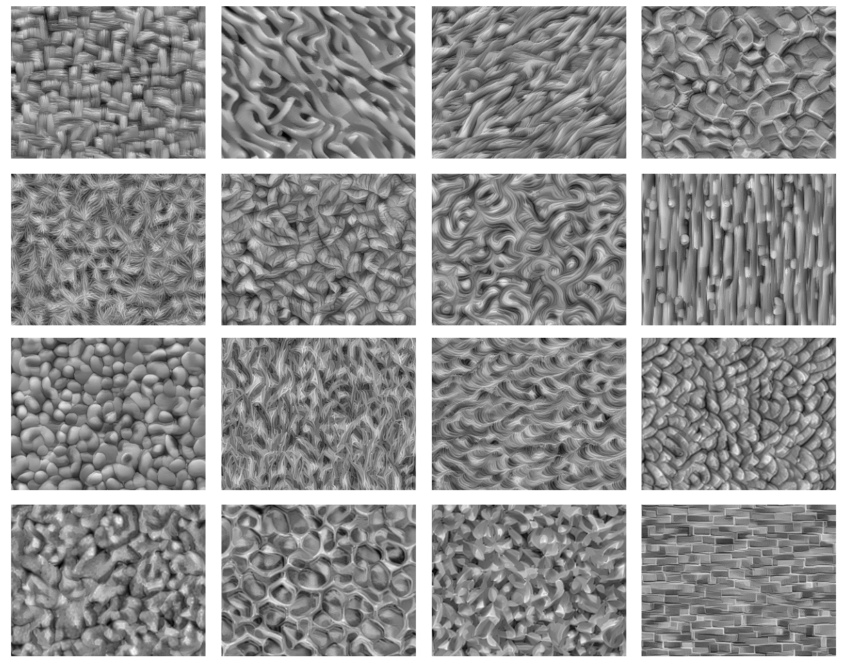

All images used in the single exemplar per family task: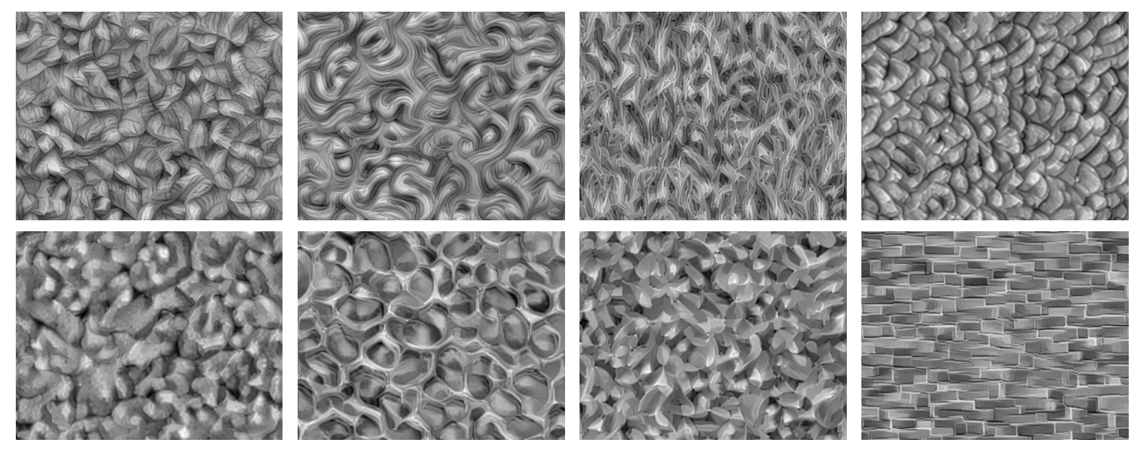

Sample of 8 exemplar images belonging to the same family (used in the Active session - multiple exemplars task). The different exemplars were obtained via random translational shifts from a reference (larger) image. The shifts were chosen to be noticeable within a V1 cell receptive field.

Environment Setup¶

⚠️Note: If running on a new environment, run this cell once and then restart the kernel⚠️

import warnings
warnings.filterwarnings('ignore')

try:
    from databook_utils.dandi_utils import dandi_download_open, dandi_stream_open
except:
    !git clone https://github.com/AllenInstitute/openscope_databook.git
    %cd openscope_databook
    %pip install -e .
    %cd docs/projects

import os

import matplotlib as mpl
import matplotlib.pyplot as plt
import numpy as np
import pandas as pd

from scipy import interpolate
from scipy.stats import ttest_ind
from math import ceil

%matplotlib inline

The Experiment¶

As shown in the metadata table below, Openscope’s Texture Project has produced 190 files on the DANDI Archive, with 9 males and 6 females. This table was generated from Getting Experimental Metadata from DANDI for textures.

session_files = pd.read_csv("../../data/texture_sessions.csv")
session_files

# Function to convert string representation of a set to an actual set
def parse_set_string(set_string):
    # Remove curly braces, split by commas, strip spaces and single quotes
    return set(item.strip("'") for item in set_string.strip("{}").split(", "))

subjects = session_files.groupby('sub_name').agg(
    n_sessions=('session_id', 'nunique'),  # Count unique session IDs
    stim_types=('stim_types', lambda x: sorted(set().union(*x.apply(parse_set_string)), reverse=True)),  # Union of all sets of stim_types
    genotype=('sub_genotype', 'unique')
).reset_index()

subjects

n_sessions = len(session_files["session_id"].value_counts())
subjects_info = session_files.groupby(["sub_name", "sub_sex"]).size().reset_index().to_dict()
m_count = len([sex for sex in subjects_info["sub_sex"].values() if sex == "M"])
f_count = len([sex for sex in subjects_info["sub_sex"].values() if sex == "F"])

print("Dandiset Overview:")
print(len(session_files), "files")
print(len(subjects_info["sub_name"]), "subjects", m_count, "males", f_count,"females")

Dandiset Overview:
144 files
15 subjects 9 males 6 females

Downloading Ophys File¶

The files can be downloaded from the DANDI Archive. For a more detailed explanation of downloading and opening these files, see Downloading an NWB file. Here, we take one file for each of the stimulus regimes used in this project; the sequentially repeated stimulus and the randomly ordered stimulus.

dandiset_id = "001461"
selected_file = 139 # 139 141 143 should allow you to test the code for every kind of session
dandi_filepath = session_files.path[selected_file]
nwb_session_type = session_files.stim_types[selected_file]
download_loc = "."
dandi_api_key = os.environ["DANDI_API_KEY"] # can be set to None if dandiset is public

# This can sometimes take a while depending on the size of the file
io = dandi_download_open(dandiset_id, dandi_filepath, download_loc, dandi_api_key=dandi_api_key)
nwb = io.read()
print("Downloaded session type: " + nwb_session_type)

File already exists
Opening file
Downloaded session type: active_single_exemplar

# view the contents of the nwb interactively
nwb

Imaging Data¶

Our Ophys files include lab metadata and imaging_planes objects which entail the information about the location being imaged, shown below. These files were chosen such that they are from the same mouse and were imaged at approximately the same depth. Note that for the 2 imaging planes within an area, the lower number corresponds to the most superficial layer, e.g., VISp_0 for layer 2/3 and VISp_1 for layer 5.

extract_depth = lambda str: str.split(" ")[3]
print("Subject ID",nwb.subject.subject_id)
for plane_name, plane in nwb.imaging_planes.items():
	print(f"{plane_name} at depth {extract_depth(plane.location)}")

Subject ID 770196
VISal_6 at depth 158
VISal_7 at depth 300
VISl_2 at depth 173
VISl_3 at depth 298
VISp_0 at depth 177
VISp_1 at depth 296
VISrl_4 at depth 173
VISrl_5 at depth 304

Extracting ROI Fluorescence¶

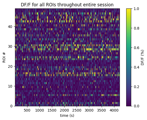
Below the 2-Photon Fluorescence data is extracted. Firstly, the imaging FOV for one session is shown with the session’s average projection, as well as the output of our cell segmentation algorithm, which identifies the cells (called regions-of-interest, or ROIs) from which the fluorescence traces were recorded. The raw fluorescence is normalized into DF/F % in order to eliminate sources of noise and day-to-day variability. The seq_dff_trace and rand_dff_trace arrays are 2D arrays pulled from the files which contain these recordings throughout the session for each ROI. They should have a shape (n_measurments x n_rois). They come with their respective arrays, seq_dff_timestamps and rand_dff_timestamps, that record the timestamp at which each measurement was taken.

plane_items = {}

for plane_name, plane in nwb.processing.items():  # iterate over string keys
    try:
        plane_items[plane_name] = (plane['images']['max_projection'], plane['images']['segmentation_mask_image'])
    except (KeyError, TypeError):
        # Skip containers that don't have 'images' or can't be indexed
        continue

n_planes = len(plane_items)
if n_planes == 0:
    print("No planes with images found.")
else:
    # Set number of columns of pairs
    n_cols = 3  # each column will be a pair of images
    n_rows = ceil(n_planes / n_cols)

    fig, axes = plt.subplots(n_rows, n_cols * 2, figsize=(6 * n_cols, 2.5 * n_rows))
    
    # Ensure axes is always 2D
    if n_rows == 1:
        axes = axes.reshape(1, n_cols * 2)

    # Flatten axes for easy indexing
    axes = axes.flatten()

    for idx, (plane_name, (max_proj, seg_mask)) in enumerate(plane_items.items()):
        # Left image of pair
        ax_left = axes[idx * 2]
        ax_left.imshow(max_proj, cmap='gray')
        ax_left.axis('off')
        ax_left.set_title(f"{plane_name} max projection", fontsize=10)

        # Right image of pair
        ax_right = axes[idx * 2 + 1]
        ax_right.imshow(seg_mask, cmap='gray')
        ax_right.axis('off')
        ax_right.set_title(f"{plane_name} segmentation mask", fontsize=10)

    # Turn off any unused axes
    for ax in axes[n_planes * 2:]:
        ax.axis('off')

    plt.tight_layout()
    plt.show()

selected_plane = "VISal_7"

dff = nwb.processing[selected_plane]["dff_timeseries"]["dff_timeseries"]
dff_trace = np.array(dff.data)
dff_timestamps = np.array(dff.timestamps)

print(dff_trace.shape)
print(dff_timestamps.shape)

avg_dff_trace = np.average(dff_trace, axis=1)

(39851, 49)
(39851,)

%matplotlib inline
n_rois = dff_trace.shape[1]
plt.imshow(dff_trace.transpose(), extent=[dff_timestamps[0], dff_timestamps[-1], 0, n_rois], aspect='auto', vmin=0, vmax=1, interpolation='None')
# plt.yticks(np.arange(n_rois)+0.5, np.arange(n_rois))
plt.ylabel("ROI #")
plt.xlabel("time (s)")
plt.title("DF/F for all ROIs throughout entire session")
cbar = plt.colorbar()
cbar.set_label('DF/F (%)')

# To check all images present and the corresponding frame
if nwb_session_type == "passive":
	for key in nwb.intervals.keys():
		print(key + " " + nwb.intervals[key].frame[0])
else:
	print("Num of stimulus presentations: " + str(len(nwb.intervals["behavior_presentations"])))

Num of stimulus presentations: 4802

Visualizing input images¶

If you want to visualize the image, they are stored in a different repository: openscope_texture_data.

import requests
from PIL import Image
from io import BytesIO 

if nwb_session_type == "passive":
    # You need to look for the image name in the list
	stim_table = nwb.intervals["fam-0-smp-3.tiff_presentations"]
	img_select = stim_table.stim_name[0] 
else:
    # Here we choose one of the X stimulus presentations instead
	img_select = nwb.intervals["behavior_presentations"]["image_name"][93] + ".tiff"

if nwb_session_type == "passive":
	img_url = "https://raw.githubusercontent.com/ComplexNSlab/openscope_texture_data/main/passive/" + img_select
elif nwb_session_type == "active_single_exemplar":
	img_url = "https://raw.githubusercontent.com/ComplexNSlab/openscope_texture_data/main/active_single_exemplar/" + img_select
elif nwb_session_type == "active_shifting_exemplars":
	img_url = "https://raw.githubusercontent.com/ComplexNSlab/openscope_texture_data/main/active_shifting_exemplars/" + img_select

    
resp = requests.get(img_url, timeout=30)
resp.raise_for_status()

im = Image.open(BytesIO(resp.content))
plt.imshow(im, cmap="gray")
plt.title(img_select)
plt.show()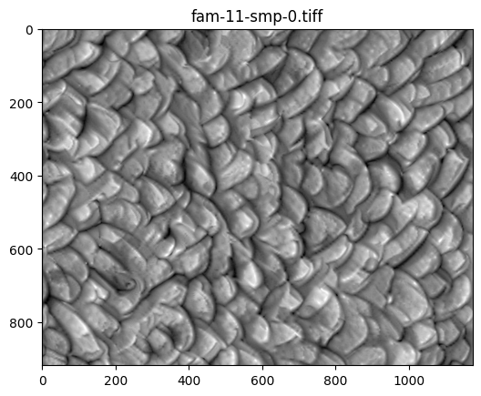

Selecting Stimulus Times¶

Stimulus information varies slighthly between active and passive seessions. In here we start with the passive sessions.

In order to analyze the data, the precise timing of the stimulus is required. This information is stored in a set of tables, one for each texture family. These are used to select trial times of interest.

Passive sessions¶

Overall, information about the stimulus is organized as follows:

There are separate folders containing timing information for each of the 16 texture families and 28 image exemplars:
‘fam-X-smp-Y.tiff_presentations’
where X goes from 0 to 15 and Y from 0 to 27.
Within each folder, there are the following lists:
‘id’: a unique integer identifying a presentation frame, runs from 0 to ~63,000
‘frame’: an integer describing which frame within the movie clip is presented this runs from -1 to 446 (-1 corresponds to family 9 stimulus 9 for some reason) ‘start_time’: time at which each frame starts this number has stretches that increment by 1/60 Hz ~ 0.01667 sec separated by larger jumps, where other stimuli are presented ‘stop_time’: time at which each frame stops; similar format to ‘start_time’
‘stim_block’: contains an integer describing the presentation order of the current movie clip this number runs from 0 to 2099. Not used
In order to find the set of times at which a given texture is presented, look for ‘start_times’ subject to the condition that ‘frame’ = frameID.

Active sessions¶

Overall, information about the stimulus is organized as follows:

Everything is contained in the same folder, called “behavior_presentations”, with one entry per stimulus presentation. Fields in there are the same as in the passive sessions.
Behavioral data is contained within the acquisition entry: “licks”, “raw_running_wheel_rotation”, “reward_volume”

# The following loads all presentations of a given stimulus
target_stim = "fam-6-smp-0"

if nwb_session_type == "passive":
	target_stim = target_stim + ".tiff_presentations"
	stim_table = nwb.intervals[target_stim]

else:
	table = nwb.intervals["behavior_presentations"]
	names = np.asarray(table["image_name"].data[:])
	idx = np.where(names == target_stim)[0]
	stim_table = table[idx]
print("Showing the first 10 presentations:")
stim_table[:10]

Showing the first 10 presentations:

To get all stimulus responses for a particular family¶

# The following loads all presentations of a given family
target_family = "fam-6"
# Needed to avoid multiple matches when checking fam-1 (since fam-10 also exists)
stim_select = lambda table_name, row: table_name.split("-smp")[0] == target_family

stim_times = []
stim_names = []
stim_frames = []
if nwb_session_type == "passive":
	table_var = nwb.intervals.items()
	for table_name, table in table_var:
		for row in table:
			if stim_select(table_name, row):
				stim_times.append(row.start_time.item())
				stim_names.append(row.name)
				stim_frames.append(row.frame.item())
else:
	table = nwb.intervals["behavior_presentations"]
	names = table["image_name"].data
	mask = np.fromiter((s.startswith(target_family) for s in names), dtype=bool, count=len(names))
	idx = np.flatnonzero(mask)
	table_var = table[idx]
	stim_times = table_var.start_time
	stim_names = table_var.name
	stim_frames = table_var.image_index


print("Selected stim times:", len(stim_times))

stim_frames_int = [int(float(t)) for t in stim_frames]

import matplotlib.pyplot as plt

plt.figure(figsize=(10,4))
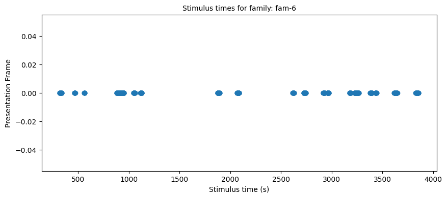
plt.plot(stim_times, stim_frames_int, 'o')
plt.xlabel("Stimulus time (s)")
plt.ylabel("Presentation Frame")
plt.title(f"Stimulus times for family: {target_family}", fontsize=10)
plt.show()

Selected stim times: 556

To get all stimulus responses to a particular exemplar¶

target_family = "fam-9-smp-0"
# Needed to avoid multiple matches when checking fam-1 (since fam-10 also exists)
stim_select = lambda table_name, row: table_name.split(".tiff")[0] == target_family

stim_times = []
stim_names = []
stim_frames = []
if nwb_session_type == "passive":
	for table_name, table in nwb.intervals.items():
		for row in table:
			if stim_select(table_name, row):
				stim_times.append(row.start_time.item())
				stim_names.append(row.name)
				stim_frames.append(row.frame.item())
else:
    # This is only useful for single exemplar active sessions
	table = nwb.intervals["behavior_presentations"]
	names = table["image_name"].data
	mask = np.fromiter((s.startswith(target_family) for s in names), dtype=bool, count=len(names))
	idx = np.flatnonzero(mask)
	table_var = table[idx]
	stim_times = table_var.start_time
	stim_names = table_var.name
	stim_frames = table_var.image_index
    
print("Selected stim times:", len(stim_times))

stim_frames_int = [int(float(t)) for t in stim_frames]

import matplotlib.pyplot as plt

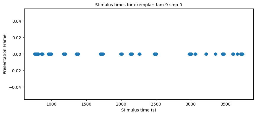
plt.figure(figsize=(10,4))
plt.plot(stim_times, stim_frames_int, 'o')
plt.xlabel("Stimulus time (s)")
plt.ylabel("Presentation Frame")
plt.title(f"Stimulus times for exemplar: {target_family}", fontsize=10)
plt.show()

Selected stim times: 658

Generating Response Windows¶

With the selected trial times above, stim_times, aligned responses to these trials throughout the session can be plotted. To align in time, the DF/F traces must first be interpolated. The code below calculates these ‘neuronwise response windows’.

window_start_time = -0.25
window_end_time = 0.75
interp_hz = 10

# generate regularly-space x values and interpolate along it
time_axis = np.arange(dff_timestamps[0], dff_timestamps[-1], step=(1/interp_hz))
interp_dff = []

# interpolate channel by channel to save RAM
for channel in range(dff_trace.shape[1]):
    f = interpolate.interp1d(dff_timestamps, dff_trace[:,channel], axis=0, kind="nearest", fill_value="extrapolate")
    interp_dff.append(f(time_axis))

interp_dff = np.array(interp_dff)

print(interp_dff.shape)

(49, 42048)

# validate window bounds
if window_start_time > 0:
    raise ValueError("start time must be non-positive number")
if window_end_time <= 0:
    raise ValueError("end time must be positive number")
    
# get event windows
windows = []
window_length = int((window_end_time-window_start_time) * interp_hz)

for stim_ts in stim_times:
    # convert time to index
    start_idx = int( (stim_ts + window_start_time - dff_timestamps[0]) * interp_hz )
    end_idx = start_idx + window_length
 
    # bounds checking
    if start_idx < 0 or end_idx > interp_dff.shape[1]:
        continue
        
    windows.append(interp_dff[:,start_idx:end_idx])
    
if len(windows) == 0:
    raise ValueError("There are no windows for these timestamps")

windows = np.array(windows) * 100 # x100 to convert values to dF/F percentage
neuronwise_windows = np.swapaxes(windows,0,1)

print(neuronwise_windows.shape)

(49, 658, 10)

Showing Response Windows¶

%matplotlib inline
def show_dff_response(ax, dff, window_start_time, window_end_time, aspect="auto", vmin=None, vmax=None, yticklabels=[], skipticks=1, xlabel="Time (s)", ylabel="ROI", cbar=True, cbar_label=None):
    if len(dff) == 0:
        print("Input data has length 0; Nothing to display")
        return

    img = ax.imshow(dff, aspect=aspect, extent=[window_start_time, window_end_time, 0, len(dff)], vmin=vmin, vmax=vmax)
    if cbar:
        ax.colorbar(img, shrink=0.5, label=cbar_label)

    ax.plot([0,0],[0, len(dff)], ":", color="white", linewidth=1.0)

    if len(yticklabels) != 0:
        ax.set_yticks(range(len(yticklabels)))
        ax.set_yticklabels(yticklabels, fontsize=8)

        n_ticks = len(yticklabels[::skipticks])
        ax.yaxis.set_major_locator(plt.MaxNLocator(n_ticks))

    ax.set_xlabel(xlabel)
    ax.set_ylabel(ylabel)

def show_many_responses(windows, rows, cols, window_idxs=None, title=None, subplot_title="", xlabel=None, ylabel=None, cbar_label=None, vmin=0, vmax=100):
    if window_idxs is None:
        window_idxs = range(len(windows))
    windows = windows[window_idxs]
    
    # handle case with no input data
    if len(windows) == 0:
        print("Input data has length 0; Nothing to display")
        return
    # handle cases when there aren't enough windows for number of rows
    if len(windows) < rows*cols:
        rows = (len(windows) // cols) + 1

    fig, axes = plt.subplots(rows, cols, figsize=(2*cols+2, 2*rows+2), layout="constrained")
    # handle case when there's only one row
    if len(axes.shape) == 1:
        axes = axes.reshape((1, axes.shape[0]))
    
    for i in range(rows*cols):
        ax_row = int(i // cols)
        ax_col = i % cols
        ax = axes[ax_row][ax_col]
        
        if i > len(windows)-1:
            ax.set_visible(False)
            continue

        window = windows[i]
        show_dff_response(ax, window, window_start_time, window_end_time, xlabel=xlabel, ylabel=ylabel, cbar=False, vmin=vmin, vmax=vmax)
        ax.set_title(f"{subplot_title} {window_idxs[i]}")
        if ax_row != rows-1:
            ax.get_xaxis().set_visible(False)
        if ax_col != 0:
            ax.get_yaxis().set_visible(False)

    fig.suptitle(title)
    norm = mpl.colors.Normalize(vmin=vmin, vmax=vmax)
    colorbar = fig.colorbar(mpl.cm.ScalarMappable(norm=norm), ax=axes, shrink=1.5/rows, label=cbar_label)

show_many_responses(neuronwise_windows,
                    6,
                    15,
                    title="Response of Some ROIs across trials",
                    subplot_title="ROI",
                    xlabel="time (s)",
                    ylabel="trial",
                    cbar_label="$\Delta$F/F (%)")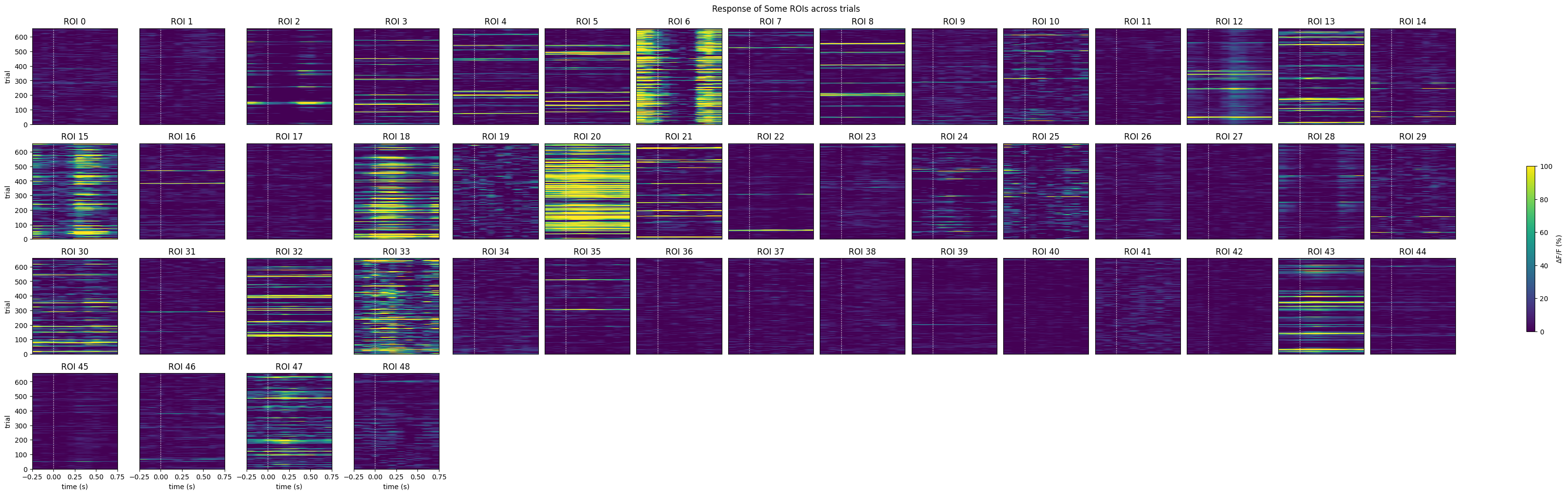

Selecting Cells¶

# get the index within the window that stimulus occurs (time 0)
stimulus_onset_idx = int(-window_start_time * interp_hz)
baseline = windows[:,:,0:stimulus_onset_idx]
evoked_responses = windows[:,:,stimulus_onset_idx:]

print(stimulus_onset_idx)
print(baseline.shape)
print(evoked_responses.shape)

2
(658, 49, 2)
(658, 49, 8)

Only keep the cells that pass the independent two-sample t-test¶

mean_trial_responses = np.mean(evoked_responses, axis=2)
mean_trial_baselines = np.mean(baseline, axis=2)

n = mean_trial_responses.shape[0]
t,p = ttest_ind(mean_trial_responses, mean_trial_baselines)
IC3_selected_rois = np.where(p < 0.05 / n)[0]
print(f"Selected ROIs {IC3_selected_rois}")

Selected ROIs [ 6 18 28]

show_many_responses(neuronwise_windows[IC3_selected_rois],
                    6,
                    15,
                    title="Response of Some ROIs across trials",
                    subplot_title="ROI",
                    xlabel="time (s)",
                    ylabel="trial",
                    cbar_label="$\Delta$F/F (%)")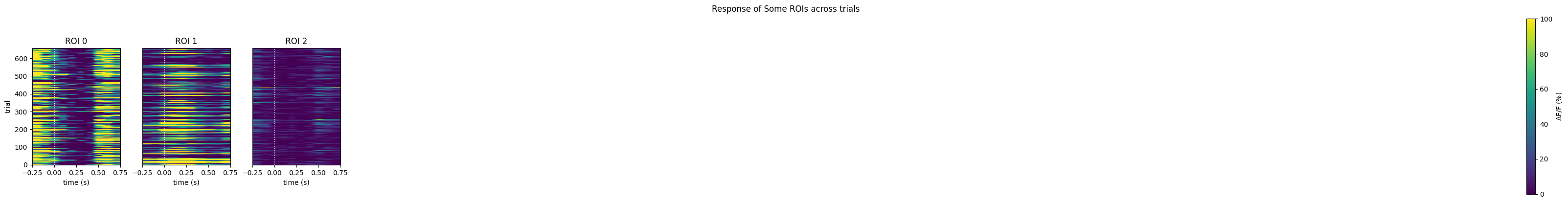

Training performance¶

The following code loads the behavioral sessions and outputs the animal performance (measured by their d’) during each session

# Calculate number of correct licks for a given session
import re
def get_correct_licks(nwb):
    lick_times = nwb.acquisition['licks'].timestamps
    img_time = nwb.intervals['behavior_presentations']['start_time']
    img_stop = img_time[-1]+.5
    img_time = np.append(img_time,img_stop)
    img_names = nwb.intervals['behavior_presentations']['image_name']
    img_fams = []
    for name in img_names:
        img_fams.append(int(re.findall(r'\d+', name)[0]))
    trans = [False]
    licks = []
    for i in range(1, len(img_fams)):
        if img_fams[i-1] == img_fams[i]:
            trans.append(False)
        else:
            trans.append(True)
    for i in range(1, len(img_time)):
        licks.append(any([img_time[i-1] < x < img_time[i] for x in lick_times]))
    true_pos = []
    for i in range(0, len(trans)):
        if trans[i] == True:
            true_pos.append(licks[i])
    return true_pos

# Moving window for the animal accuracy
def moving_accuracy(trials, window=25):
    mov_avg = []
    for i in range((window//2), len(trials)-(window//2)):
        samp = trials[i-(window//2):i+(window//2)]
        win_avg = np.mean(samp)
        mov_avg.append(win_avg)
    return mov_avg

# Concatenate performance across multiple sessions
def plot_all_tp(nwb_list, window=25):
    true_pos_ses = []
    ses_means = []
    ses_lens = [0]
    for nwb in nwb_list:
        try:
            print(f"Processing file: {nwb.session_id}")
            tp = get_correct_licks(nwb)
            ma = moving_accuracy(tp, window)
            true_pos_ses+=ma
            ses_means+=[np.mean(tp)]*len(ma)
            ses_lens.append(len(ma))
        except KeyError:
            pass
    sum_lens = np.cumsum(ses_lens)
    for l in sum_lens[:-1]:
        plt.axvline(x=l, color='k', linestyle='--', alpha=0.5)
    plt.plot(true_pos_ses)
    plt.plot(ses_means)
    plt.xlabel('trial number')
    plt.ylabel('running average performance')
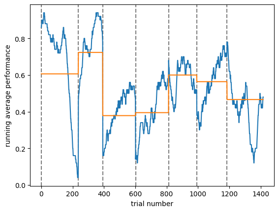
    plt.show()

Animal performance across multiple sessions¶

First choose a specimen from the original list and download all nwb files related to active sessions. Sort the files chronologically.

specimen = 762551

# Get all sessions, remove passive and sort chronologically
mask = session_files["sub_name"] == specimen
session_info = session_files.loc[session_files["sub_name"] == specimen, ["path", "stim_types", "session_time"]]
session_info["session_time"] = pd.to_datetime(session_info["session_time"])
session_info = session_info.sort_values("session_time")
session_info = session_info[session_info["stim_types"] != "passive"]
#print(session_info)

nwb_list = []
ct = 0

for idx, row in session_info.iterrows():
    print(f"Loading NWB {ct+1}/{len(session_info)}")
    io = dandi_stream_open(dandiset_id, row["path"], dandi_api_key=dandi_api_key)
    nwb = io.read()
    nwb_list.append(nwb)
    ct += 1
print(f"Loaded {ct} nwb files")

Loading NWB 1/7
Loading NWB 2/7
Loading NWB 3/7
Loading NWB 4/7
Loading NWB 5/7
Loading NWB 6/7
Loading NWB 7/7
Loaded 7 nwb files

# This will concatenate all sessions and plot a within session moving average (and session average) performance thbroughout the sessions
plot_all_tp(nwb_list, window=50)

Processing file: multiplane-ophys_762551_2025-01-16_14-30-36
Processing file: multiplane-ophys_762551_2025-01-21_12-04-09
Processing file: multiplane-ophys_762551_2025-01-23_15-07-09
Processing file: multiplane-ophys_762551_2025-01-24_14-19-46
Processing file: multiplane-ophys_762551_2025-01-27_10-07-52
Processing file: multiplane-ophys_762551_2025-01-28_11-31-36
Processing file: multiplane-ophys_762551_2025-01-29_09-46-34