Examples (dipde.examples)
These quick-start examples demonstrate the configuration, simulation, and plotting of simple dipde networks.
A preamble imports the classes necessary for simulation:
import matplotlib.pyplot as plt
from dipde.internals.internalpopulation import InternalPopulation
from dipde.internals.externalpopulation import ExternalPopulation
from dipde.internals.simulation import Simulation
from dipde.internals.connection import Connection as Connection
Each of the example simulations below use the same general settings:
# Settings:
t0 = 0.
dt = .0001
dv = .0001
tf = .1
update_method = 'approx'
approx_order = 1
tol = 1e-14
verbose = True
Here dt defines the time step of the simulation (in seconds), dv defines the granularity of the voltage domain of the Internal populations (in volts), and tf defines the total duration of the simulation (in seconds). The update method allows the user to change the time-stepping method for the forward evolution of the time domain of each Internal population. The approx_order and tol options fine-tune the time stepping, to provide a tradeoff between simulation time and numerical precision when the time evolution method is ‘approx,’ as opposed to ‘exact.’ Setting verbose to True causes the Simulation to print the current time after the evaluation of each time step.
Singlepop
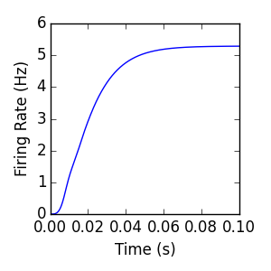
The singlepop simulation provides a simple feedforward topology that uses every major class in the core library. A single 100 Hz External population population (here specified as a string, although a floating point or integer specification will work also) provides excitatory input. This is connected to an Internal population (modeled as a population density pde) via a delta-distributed synaptic weight distribution, with 5 mV strength. The in-degree (nsyn) of this Connection is set to 1 for this example; in general, this serves as a multiplier of the input firing rate of the source population. The internal population has a linearly binned voltage domain from v_min to v_max. No negative bins (i.e. v_min < 0) are required here, because no negative synaptic inputs (‘weights’ in the Connection object) are defined.
# Create simulation:
b1 = ExternalPopulation('100', record=True)
i1 = InternalPopulation(v_min=0, v_max=.02, dv=dv, update_method=update_method, approx_order=approx_order, tol=tol)
b1_i1 = Connection(b1, i1, 1, weights=[.005], probs=[1.], delay=0.0)
simulation = Simulation([b1, i1], [b1_i1], verbose=verbose)
simulation.run(dt=dt, tf=tf, t0=t0)
- The mean firing rate of the Internal population resulting from this simulation is
- plotted below, along with the code used to generate the plot:
# Visualize:
i1 = simulation.population_list[1]
plt.figure(figsize=(3,3))
plt.plot(i1.t_record, i1.firing_rate_record)
plt.xlim([0,tf])
plt.ylim(ymin=0)
plt.xlabel('Time (s)')
plt.ylabel('Firing Rate (Hz)')
Singlepop (recurrent)
Download singlepop_recurrent.py
The next example is identical to the singlepop example, with the exception of an additional recurrent connection from the internal population to itself. This demonstrates that the Connection object is used to connect both Internal and External population sources to an Internal target population. Attempting to create a Connection with an External population as a target will result in an AttributeError. The additional excitatory input resulting from the extra recurrent connection results in a slightly increased steady-state firing rate.
# Create simulation:
b1 = ExternalPopulation('100')
i1 = InternalPopulation(v_min=0, v_max=.02, dv=dv, update_method=update_method, approx_order=approx_order, tol=tol)
b1_i1 = Connection(b1, i1, 1, weights=[.005], probs=[1.], delay=0.0)
i1_i1 = Connection(i1, i1, 1, weights=[.005], probs=[1.], delay=0.0)
simulation = Simulation([b1, i1], [b1_i1, i1_i1], verbose=verbose)
simulation.run(dt=dt, tf=tf, t0=t0)

Excitatory/Inhibitory
Download excitatory_inhibitory.py
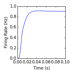
Inhibitory connections are formed the same as excitatory connections, except the sign of the connection weight distribution is changed. In this example, the background External population is connected to the Internal population with two connections, one excitatory and one inhibitory. Because of this negative input, negative voltage values are possible, requiring that v_min<0.
b1 = ExternalPopulation('100')
i1 = InternalPopulation(v_min=-.02, v_max=.02, dv=dv, update_method=update_method, approx_order=approx_order, tol=tol)
b1_i1 = Connection(b1, i1, 1, weights=[.005], probs=[1.], delay=0.0)
b1_i1_2 = Connection(b1, i1, 1, weights=[-.005], probs=[1.], delay=0.0)
simulation = Simulation([b1, i1], [b1_i1, b1_i1_2],  verbose=verbose)
simulation.run(dt=dt, tf=tf, t0=t0)
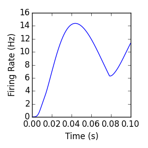
Singlepop (sine)
By modifying the argument to the ExternalPopulation constructor, we can define a time-varying external input. This input is parsed by Sympy using the lambdify module; any lambdify-able expression with the independent variable ‘t’ is acceptable. Negative values of the firing rate function will throw an Exception.
# Create simulation:
b1 = ExternalPopulation('100+50*abs(sin(40*t))')
i1 = InternalPopulation(v_min=0, v_max=.02, dv=dv, update_method=update_method, approx_order=approx_order, tol=tol)
b1_i1 = Connection(b1, i1, 1, weights=[.005], probs=[1.], delay=0.0)
simulation = Simulation([b1, i1], [b1_i1], verbose=verbose)
Singlepop (exponential)
Download singlepop_exponential_distribution.py
Up until now, each connection object was defined with a single synaptic weight. However, connection objects are fundamentally defined by synaptic weight distributions (See Iyer et al. 2013 [1]). Here we consider the effect of an exponentially distributed synaptic weight distribution with mean equal to 5 mV. The steady state firing rate under this stimulus is significantly higher than the delta-distributed example (singlepop, above). In general, any Continuous synaptic weight distribution can be defined using scipy.stats module; however it will be discretized into a finite set of input weights. Discrete distributions can be specified directly, and will be used exactly.
import scipy.stats as sps

# Create simulation:
b1 = ExternalPopulation(100)
i1 = InternalPopulation(v_min=0, v_max=.02, dv=dv, update_method=update_method, approx_order=approx_order, tol=tol)
b1_i1 = Connection(b1, i1, 1, delay=0.0, distribution=sps.expon, N=201, scale=.005)
simulation = Simulation([b1, i1], [b1_i1], verbose=verbose)
simulation.run(dt=dt, tf=tf, t0=t0)
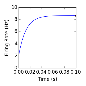
In general, the special case of exponentially distributed synaptic weights admits an analytical steady-state firing rate solution (see Richardson and Swarbrick, 2010 [2], and Iyer et al. 2014 [3]). The figure above includes the mean firing rate computed for the internal population, as well as a ‘*’ indicating a semi-analytic prediction (~8.669 Hz) of the steady-state firing rate for the model. This steady state prediction is computed with the code below, plotted above with an ‘*’.
import scipy.integrate as spint
import numpy as np

R_e = 100
a_e = .005
tau = .02
v_th = .02
f = lambda c: (1./c)*(1-a_e*c)**(tau*R_e)*(np.exp(v_th*c)/(1-a_e*c)-1.)
y, _ = spint.quad(f,0.0,1./a_e)
steady_state_prediction = 1./(tau*y)    # >>> 8.6687760498
| [1] | Iyer, R., Menon, V., Buice, M., Koch, C., & Mihalas, S. (2013). The Influence of Synaptic Weight Distribution on Neuronal Population Dynamics. PLoS Computational Biology, 9(10), e1003248. doi:10.1371/journal.pcbi.1003248 |
| [2] | Richardson, Magnus J. E. & Swarbrick, Rupert (2010). Firing-Rate Response of a Neuron Receiving Excitatory and Inhibitory Synaptic Shot Noise. Phys. Rev. Lett., 105, 178102. |
| [3] | Iyer, R., Cain, N., & Mihalas, S. (2014). Dynamics of excitatory-inhibitory neuronal networks with exponential synaptic weight distributions. Cosyne Abstracts 2014, Salt Lake City USA. |